Visualizing Dynamics Using the Multi Frame FLIM Analysis (updated for SymPhoTime v2.5 and above)

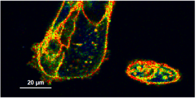
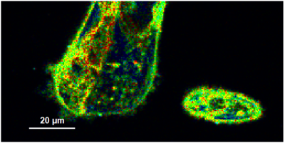
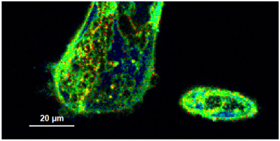
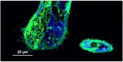
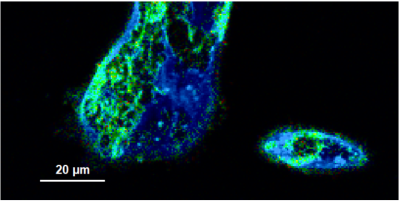
This tutorial shows step-by-step, how to separate the different frames of multi-frame image with systems equipped with a fast Galvo scanner. The image containing many frames is treated here like a time-series. The example image shows the plasma membrane of MDCK cells stained with Flipper-TR, which can report membrane tension changes through its fluorescence lifetime changes. This has been published 2018 in nature: https://www.nature.com/articles/s41557-018-0127-3. This dynamics is visualized with the “multi Frame FLIM” script. Only few of the frames are binned together for analysis, and an image series is obtained. The lifetime change will be monitored at the end.

Tutorials workspace can be downloaded from https://figshare.com/s/4957fcfa684daef86c23.

• Start SymPhoTime 64 software (this tutorial uses version 2.5).
• Open the “Tutorials” workspace via File → Open Workspace from the main menu.
  

Response:​
​ The files of the “Tutorials” workspace are displayed in the workspace panel on the left side of the main window.

• Highlight the file Hyperosmotic_Shock_MDCK_Cells.ptu ​by a single mouse click.
• Select the “​Analysis”​ tab and in there, open the “​Imaging”​ drop-down menu.
  
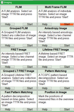
• Start the “multi Frame FLIM” analysis by clicking on “Start”.
  

Response:​
​ The FLIM analysis is applied to the file Hyperosmotic_Shock_MDCK_Cells.ptu. Thereby, a new Window opens:

Note:
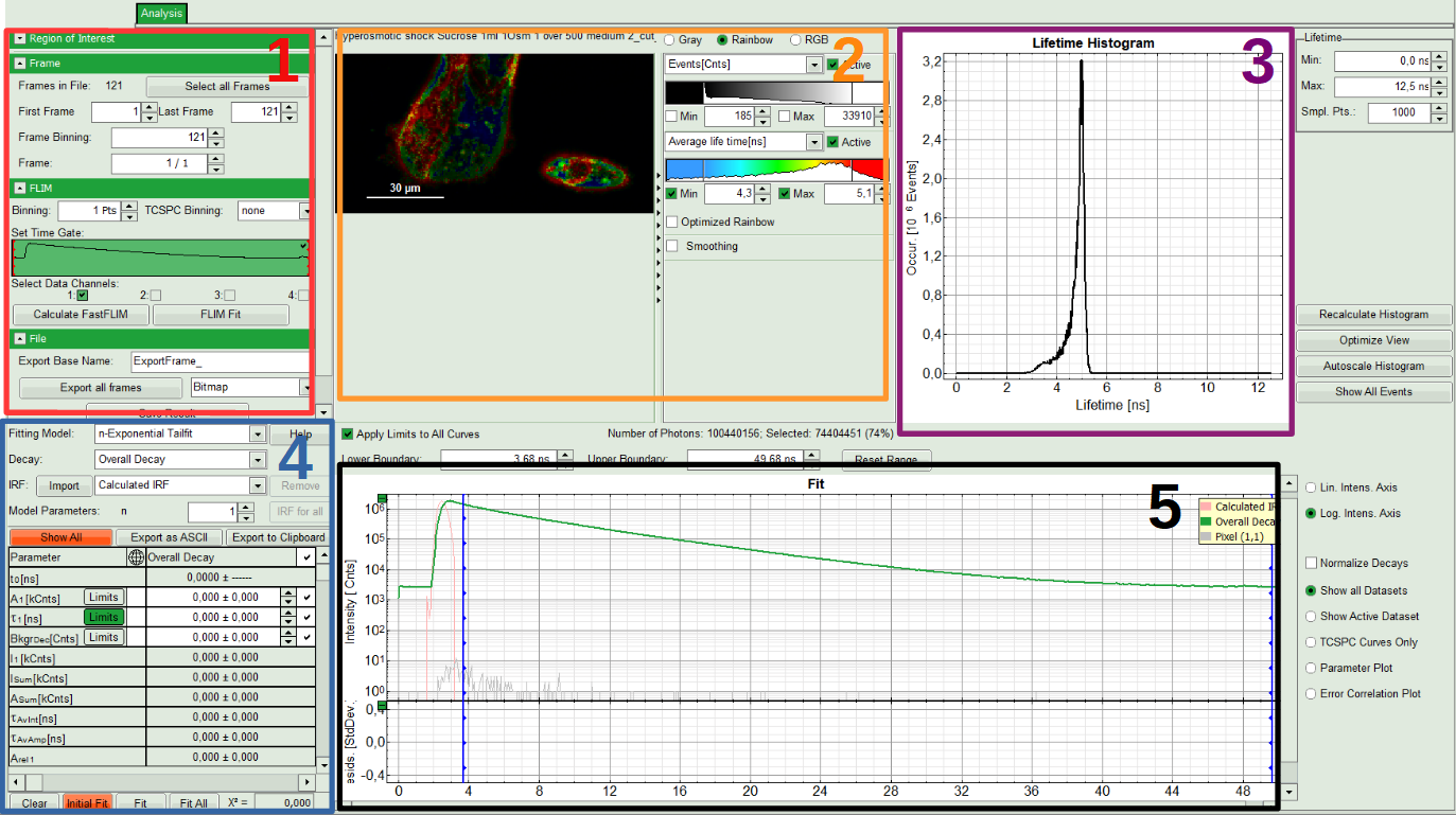
The window contains five different sections:
1: Setting panel
Imaging analysis options can be defined in this section.
2: Fast FLIM image
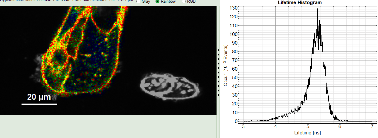
The FLIM preview image displayed in a false color scale. The brightness encodes the intensity, while the color encodes the average “Fast FLIM” lifetime, i.e. the mean arrival times of the photons after the laser pulse. When not defined otherwise, intensity and color scale stretch from minimum to maximum. As the mean arrival time of the background photons in the areas where no fluorescence is detected, is randomly spread over the TCSPC window, the mean photon arrival time of the dark background is usually very long (with an average up to 1/2 of the TCSPC window), which makes the color scale loaded by default sometimes unsuited for displaying the lifetime contrast in the actual sample. In this case, the scale can be adapted.
3: Fluorescence Lifetime Histogram
Here the frequency of photon counts corresponding to the individual mean lifetimes is plotted. The settings of the plot can be adapted using the controls on the right of the plot. The histogram is photon weighted.
4: Decay Fitting Parameters
Here the lifetime fitting model can be selected. Fitting is then applied to the lifetime graph(s) on the lower center (TCSPC histogram).
5: TCSPC Decay window​
By default, this set shows the TCSPC histogram of all photons in the image in green (= dataset 0) and the TCSPC histogram of a single pixel in grey (= dataset 1). In red an estimation of the instrument response function (=IRF) is shown. The IRF reconstruction is deducted from the rising edge of the TCSPC histogram.

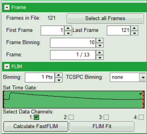
• In parameter panel, enter a frame binning of 10 in order to decrease processing time and increase photon numbers per pixel, while still visualizing the temporal changes. Then start the recalculation by clicking on “Calculate FastFLIM”.
  

Response:
An image stack is calculated, in which always 10 frames are combined. As the complete measurement contains 121 frames, the image stack now contains 13 images.

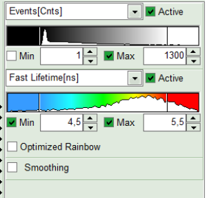
• To enhance the lifetime contrast, adapt the color scale by typing the limit values for the “Fast Lifetime [ns]” and “Events[cnts]”. Additionally set the “Lifetime Histogram” range on the right hand.
  

• You can scroll through the images by walking through the number displayed at “Frame” using the arrows next to the numbers.
• A few images of the series is plotted here; images 1 [Frame 1-10], 3 [Frame 21-30], 4, 6, 10:
  

Note:
Flipper-TR is a fluorescent probe that specifically targets the plasma membrane of cells which sense changes of the organization of lipid bilayer membranes through changes of the twist angle and polarization between the two twisted dithienothiophenes of the mechanophore.

• While you could export the images via “Export all Frames” in the “File”-menu, here we will now illustrate here how to visualize the lifetime change at the certain ROI.

• Right click on the FastFLIM image and from the context menu select “FreeROI” tool.
  

• In order to quantify tension changes in cell membrane, draw a ROI on the image where the bigger cells are located.

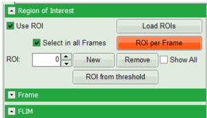
• Tick the “Select in all Frames” checkbox. Click “ROI per Frame” to select an ROI with the same marked pixels in each frame.
  

Response:
When the ROI in each image is created, also the corresponding decay appears in grey in the TCSPC decay window.

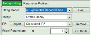
• In the “Decay Fitting” panel, from the Fitting Model drop-down list select “n-Exponential Reconvolution Fit”.
  

Response:
In the TCSPC window, the IRF is displayed in bright red, the data fitting limits are moved to the borders of the TCSPC window.
The new fitting parameters “Shift IRF” and “Bkgr IRF” (=background IRF) appear in the fitting parameter table.

Note:
The software offers the possibility to fit the data using a n-exponential tail fit, n-exponential reconvolution or rapid reconvolution fit. A tail fit can be used when the fitted lifetimes are significantly longer than the instrument response function. A reconvolution fit is usually preferable, because the complete decay is fitted, while for a tail fit, the start of the fitting range is usually a bit arbitrary.

For explanation about the fitting model and the used equations, click on the “Help” button next to the selected model. This opens a help window containing the fitting equation and the explanation of the different parameters.

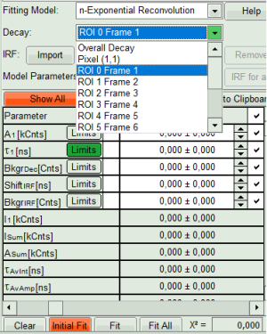
• From “Decay” drop-down list select ROI 0 and click “Initial Fit” (marked in orange).
  

Response:
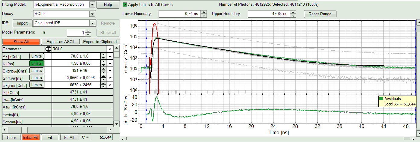
A single exponential reconvolution fit is performed. In the TCSPC window, the fit is displayed as a black line. Below, the residuals (= difference between raw data and fit values) are displayed.

• Fit values appear in the fitting table. Check the fitting curve, residuals and χ².
  

Note:

Usually, a decent fit is characterized by the following criteria:

1. The fitted curve overlays well with the decay curve. In the residual window, the values spread randomly around 0.
   
2. The χ²-value approaches 1.
   
3. The calculated fitting values are reasonable.
   
4. The fitting model with least parameters is preferred.
   

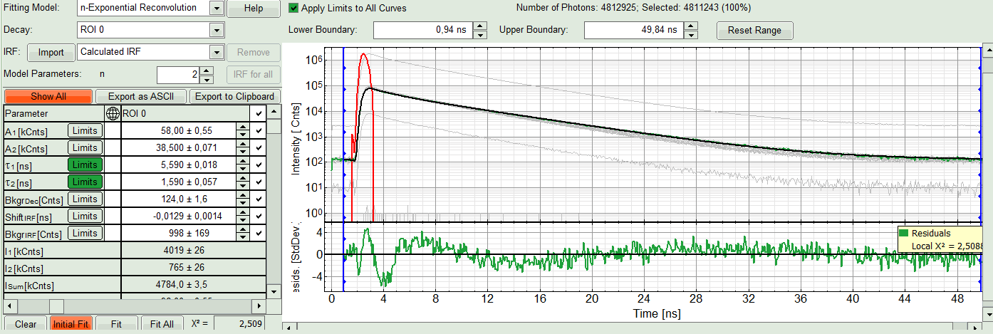
• In this example it is obvious that the applied single exponential reconvolution fit is not suited to fit the decay curve. Increase the “Model Parameters” to n = 2. Again, click on “Initial fit”.
  

Response:
The fit quality increases. But if it still doesn't look sufficient, increase number of “Model Parameters” to three.

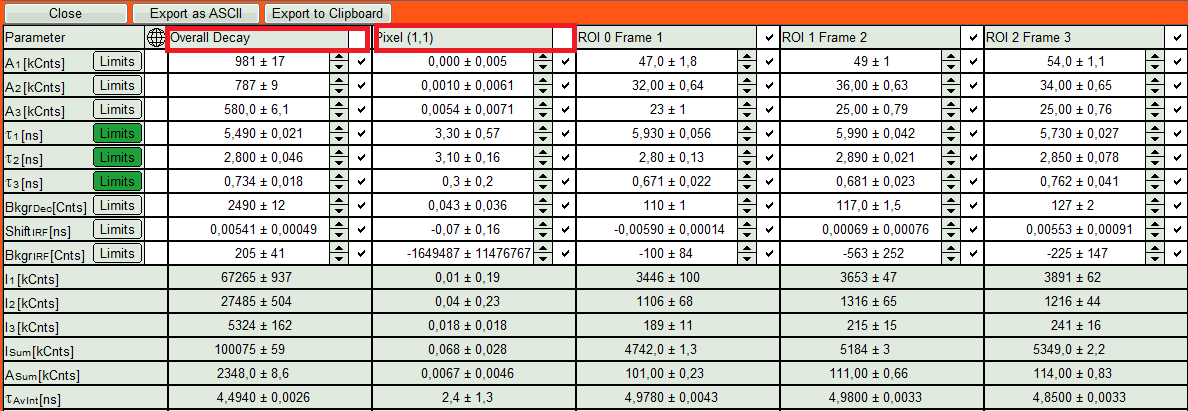
• We apply fit now all ROIs using the fitting model and start parameters from the ROI0-fit by pressing “Fit All”.

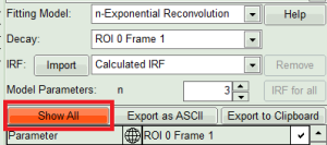
• The fit results for all datasets can be seen (and exported) as a table using the “Show all”-button.
  

• Clicking on “Fit All” will fit all active data sets with the same model, using the start parameters of the active data set. If you do not want to fit the complete decay (dataset 1) and the decay of a single pixel (Dataset 2), press “Show All” button, uncheck the first two datasets on top of the parameter table and press “Fit All” again.
  

Response:

• On the right hand of the TCSPC window select “Parameter Plot” to get a graphical impression of the change of the fit values and compare for instance average lifetime of your ROIs.

• Select the intensity averaged lifetime for the Y-Axis; tick the “tau_Av_In” checkbox and deselect the unwanted fitting parameters.

Response:
The average lifetime, you can see that after adding the sugar, has been dropped gradually about 500ps.

• If an IRF has been measured, the fits can also be performed using the measured IRFs. You need to import your measured IRF for the respective channel. Then repeat the above steps to find a decent fit. For more details please see How to Work with Instrument Response Functions (IRFs) Measured with a Microscope.
  

• Click on “Export all frames” with the selection “Bitmap”.

Note:
There are several options to export the data:

1. Bitmap exports the image as a bmp file. If the scale bar is displayed, the image including the scale bar is exported.
2. Bitmap with color scale exports the image as a bmp file including the intensity and color scale next to the image.
3. 1×1 bitmap exports the image as a bmp file with one pixel of the image being exported as one pixel in the image file. In the other bitmap export options, the image is exported as displayed.
4. ASCII exports the image as an ASCII array using a text-file format. Thereby one array encodes the intensity values, while a second array encodes the Fast Lifetime values. If a pixel-by-pixel fit has been performed, there are more arrays depending on the fitting model used. After removal of the header and the unwanted array, individual arrays can be imported in graphic programs, e.g. ImageJ as a text image. These images contain the full count resolution of the raw image.
5. TIFF exports the image series as a series of 32 bit tiff-files, which can be opened e..g using open source software like Fiji
   
6. BIN exports the image series as a series of binary files. The data format of these files is described on the SymPhoTime Online help. The binary files contain the photon information of each TCSPC-channel and can be imported e.g. in Phasor Plot analysis routines.

• A window opens asking for a place and name to store the images. Create a folder and save the images.
  

Response:
26 images are exported as .bmp files into this folder. You can import them into other graphic programs, e.g. Fiji, in order to create movies.

Note:
When exporting as standard bitmap, the images are exported as shown in the SymPhoTime 64 window, e.g with or without scale bar (depending on whether you have the scalebar active in the SymPhoTime. When measuring with a scanner controlled by SymPhoTime, e.g. a MicroTime system, or you transfer the image size information automatically via a handshake software, as in several LSMs, the image size is automatically adapted. If your scanner is not controlled via the SymPhoTime, and no handshake transfers the correct image size correctly, the image size has to be checked and if it is necessary defined before the measurement. Otherwise, one pixel is considered to a size of 1 µm. If the image scaling should not be displayed, put the mouse cursor over the image, open the context menu with a right mouse click and unselect the option “Show Scale-bar”. When the scale bar is not displayed, the exported images also do not contain the scale bar.

Note:

If not only the Fast FLIM image should be exported, but also a pixel-by-pixel fit for the whole stack is needed, a procedure according to the tutorial: “Lifetime fitting using the FLIM script” must be applied. Please follow the instructions as described there in an analogous fashion.

• Finally, store the analysis results by clicking “Save Results”.
  

Response:
A result file is generated which is assigned to the raw data file. Double click on this .pqres-file opens it in the same way as it was stored.