Visualizing Dynamics Using the Multi Frame FLIM Analysis
Summary
This tutorial shows step-by-step, how to separate the different frames of a multi frame image typically acquired with systems containing a fast Galvo scanner. In this tutorial, an image showing partially moving giant unilaminar vesicles (GUVs) is processed with the multi frame FLIM script. Only a few subframes are combined for analysis. The result is exported as an image series.
Step-by-Step Tutorial
Select a file and start the script
- Start SymPhoTime 64 software.
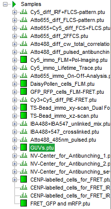
- Open the “Samples” workspace via “File → Open Workspace” from the main menu.
Note: The “Samples” workspace is delivered with the SymPhoTime 64 and on the CD-ROM and contains example data to show the function of the SymPhoTime data analysis. If you haven't installed it on your computer, copy it from the DVD onto a local drive before going through this tutorial.
Response: The files of the sample workspace are displayed in the workspace panel on the left side of the main window.
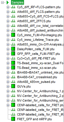
- Highlight the file
GUVs.ptuby a single mouse click.
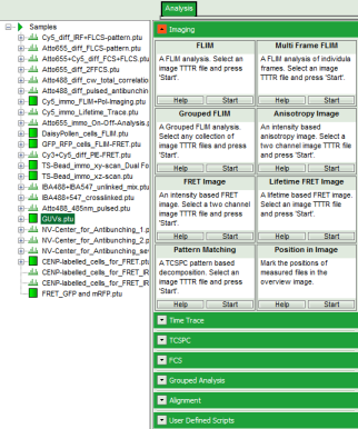
- Select the “Analysis” tab and in there, open the drop down menu “Imaging”.
Note: The drop down menu can be opened and closed by clicking on the grey button on the left side of the header of the drop down menu: 
- Start the “Multi Frame FLIM” script by clicking on “Start”.
Response: The “Multi Frame FLIM” script is applied to the file GUs.ptu. Thereby, a new Window opens:
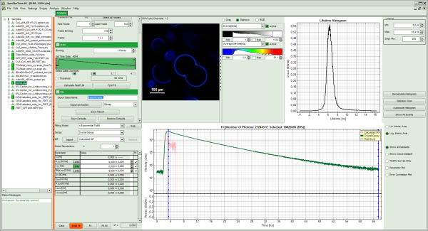
Note: The window contains five different regions:
- Upper left: Imaging analysis options. As there are many options in this panel, not all of them fit into the visible area of the screen. Thus, a scroll bar is generated to access all controls.
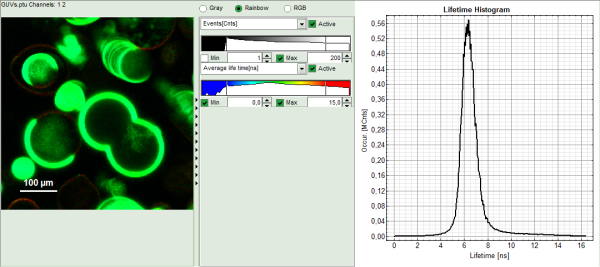
- Upper center: Fast FLIM image displayed in false color scale. The brightness encodes the intensity while the color encodes the average “Fast FLIM” lifetime, i.e. the mean arrival times of the photons after the laser pulse. When not defined otherwise, intensity and color scale stretch from minimum to maximum. As the mean arrival time of the background photons in the areas where no fluorescence is detected, is randomly spread over the TCSPC window, the mean photon arrival time of the dark background is usually very long (up to 1/2 of the TCSPC window), which makes the color scale loaded by default sometimes unsuited for displaying the lifetime contrast in the actual sample. In this case, the scale has to be adapted.
- Upper right: Fluorescence Lifetime Histogram. Here the frequency of photon counts corresponding to the individual mean lifetimes is plotted. The settings of the plot can be adapted using the controls on the right of the plot.
- Lower left: Lifetime fitting parameters allowing to define the lifetime fitting models. Fitting is then applied to the lifetime graph(s) in the TCSPC histogram.
- Lower center/left: TCSPC histogram of all photons in the image in green (= dataset 0) and the TCSPC histogram of a single pixel in grey (= dataset 1). In red an estimation of the instrument response function (= IRF) is shown. The IRF reconstruction is deducted from the rising edge of the TCSPC histogram.
- To enhance the lifetime contrast within the image, adapt the color scale from 0 to 15 ns by typing these values as limits for the Fast Lifetime color scale. Also adjust the intensity scale to 1 – 200 counts.
Note: Reasonable limits can either be found by dragging the limit bars in the color scale “Fast Lifetime” histogram or by considering the peaks of the “Lifetime Histogram”. Entering fixed values has the advantage that different images can be compared later.
Response: The intensity and color scale in the image adapt.
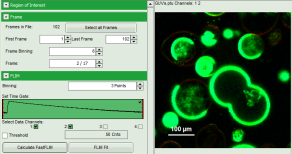
Note: The image shows giant unilaminar vesicles (GUVs) labeled with a lipid labelled derivative of nitrobenzoxadiazole (NBD). This dye has a longer lifetime when incorporated into the ordered domains of the GUVs compared to the – much stronger – incorporation into the disordered domains. For demonstration purpose of this tutorial, the most important feature of the image is that not all GUVs are completely stationary during the imaging process indicated by blurring of certain GUVs.
Select the Processing Options and create and export an image stack
Note: The fitting parameter table indicates that the image consists of 102 individual frames. By default, a frame binning of 102 is selected. Thus, the measurement is plotted as one image containing all frames.
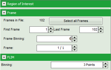
- Shift the parameter pannel up and enter a frame binning of 6 and a (pixel) binning of 3 to decrease processing time and increase photon numbers per pixel.
- Start the recalculation by clicking on “Calculate FastFLIM”.
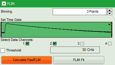
Note: The image contains data from two detectors, and both are selected for analysis. In this measurement, the fluorescence was separated by polarization, therefore, photons from both channels can be included for lifetime calculation.
Response:
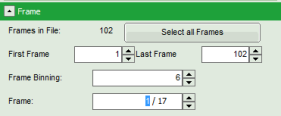
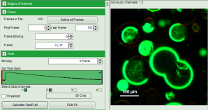
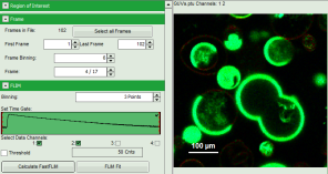
- An image stack is calculated according to the set pixel binning, in which always 6 frames are combined. As the complete measurement contains 102 frames, the image stack now contains 17 images. The first image of the series is plotted.
- One can click through the images using the control arrows in the “Frame” control. This changes the displayed frame (marked in blue).
⇓
⇓
⇓
⇓
…
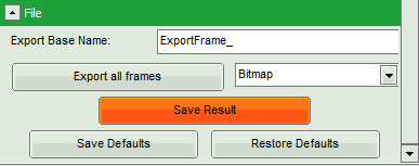
- Click on “Export all frames” with the selection “Bitmap”.
Note: There are several options to export the data:
Bitmap exports the image as a bmp file. If the scale bar is displayed, the image including the scale bar is exported.
Bitmap with color scale exports the image as a bmp file including the intensity and color scale next to the image.
1×1 bitmap exports the image as a bmp file with one pixel of the image being exported as one pixel in the image file. In the other bitmap export options, the image is exported as displayed.
ASCII exports the image as an ASCII array using a text-file format. Thereby one array encodes the intensity values, while a second array encodes the Fast Lifetime values. If a pixel-by-pixel fit has been performed, there are more arrays depending on the fitting model used. After removal of the header and the unwanted array, individual arrays can be imported in graphic programs, e.g. ImageJ as a text image. These images contain the full count resolution of the raw image.
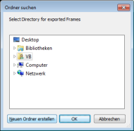
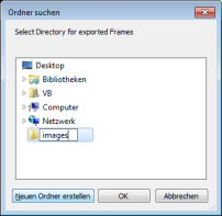
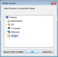
- A window opens asking for a place and name to store the images. Create a folder and save the images.
⇓
⇓
Response: 17 images are exported as .bmp files into this folder. One can import them into other graphic programs, e.g. to create movies.
Note: The images are exported as shown in the SymPhoTime 64 window, e.g. including the scale bar. If data are acquired with a scanner controlled by the SymPhoTime 64 software (i.e. the piezo scanner in the MicroTime200), the image dimensions are automatically correct. If the image is acquired using an external scanner, the image size has to be defined or transferred before the measurement to make sure that the measured image dimensions are correct. Otherwise, one pixel is considered to a size of 1 µm. If the image scaling should not be displayed, put the mouse cursor over the image, open the context menu with a right mouse click and unselect the option “Show ScaleBar”. When the scale bar is not displayed, the exported images also do not contain the scale bar.
- Shift the scroll bar at the parameter controls down and click on “Save Results” to store the data.
Response: A result file is generated which is assigned to the raw data file. Double click on this .pqres file opens it in the same way as it was stored.
Perform a FLIM Fit
Note: If not only the Fast FLIM image should be exported, but also a pixel-by-pixel fit for the whole stack is needed, a procedure according to the tutorial: Lifetime fitting using the FLIM Analysis must be applied. Please follow the instructions as described there in an analogous fashion:
- Fit the fluorescence decay and determine the fitting model and parameters.
- Set the minimum intensity threshold.
- Start the “FLIM Fit”.
When performing a pixel-by-pixel fit in the “Multi Frame FLIM” script, keep in mind that many more pixels as usual need to be fitted. In this example, 17 images have to be analyzed, which can be quite time consuming. Therefore, it can be helpful to limit the number of calculated pixels via ROI selection. The usage of the ROI selection tools is described in the script ROI fitting using the FLIM script.
By default, the ROI is only applied to the displayed image, and not to all other images in the stack. If the ROI should be used in all images of the series, first check “Select in all Frames” and then mark the ROI.
