Lifetime Fitting Using the FLIM Analysis
Summary
This tutorial shows step-by-step, how the FLIM analysis of SymPhoTime 64 can be used to perform a lifetime fit and how to extract and read the results. In detail, the FLIM analysis is started using a daisy pollen image in the “Samples” workspace, a suited fitting model is chosen and a pixel-by-pixel fit is performed.
Step-by-Step Tutorial
Select a file and start the analysis
- Start SymPhoTime 64 software
- Open the “Samples” workspace via “File\open Workspace” from the main menu.
Note:
The “Samples” workspace is delivered with the SymPhoTime 64 and on the DVD-ROM drive and contains example data to show the function of the SymPhoTime 64 data analysis. If you haven't installed it on your computer, copy it from the DVD onto a local drive before going through this tutorial.
Response:
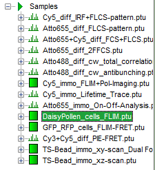
The files of the sample workspace are displayed in the workspace panel on the left side of the main window.
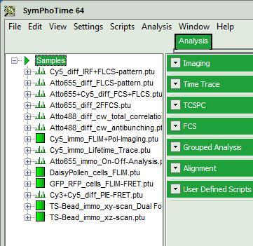
- Highlight the file DaisyPollen_cells_FLIM by a single mouse click.
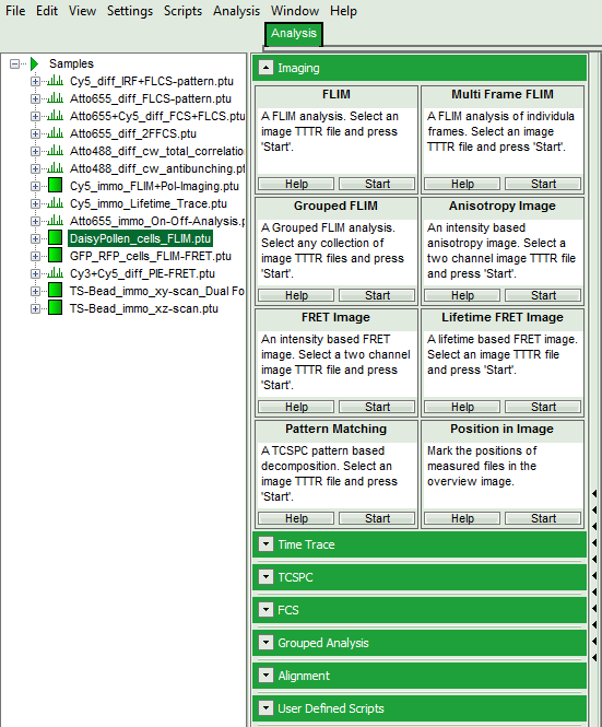
- Select the “Analysis” tab and in there, open the drop down menu “Imaging”.
Note:
The drop down menu can be opened and closed by clicking on the grey button on the left side of the header of the drop down menu: 
- Start the FLIM analysis by clicking on “Start”.
Response:
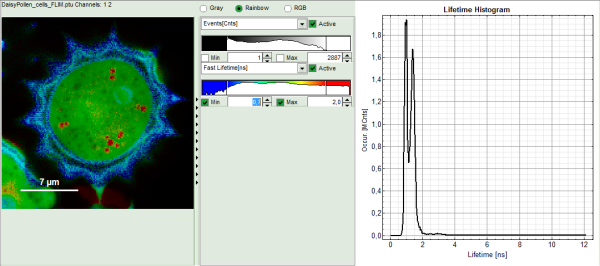
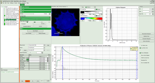
The FLIM analysis is applied to the file DaisyPollen_cells_FLIM.ptu. Thereby, a new Window opens:
Note:
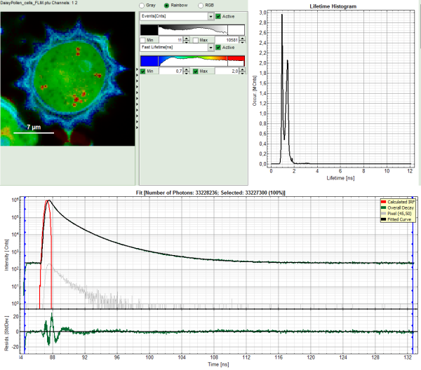
The window contains five different regions:
Upper left: imaging analysis options.
Upper center: Fast FLIM image, displayed in a false color scale. The brightness encodes the intensity while the color encodes the average “Fast FLIM” lifetime, i.e. the mean arrival times of the photons after the laser pulse. When not defined otherwise, intensity and color scale stretch from minimum to maximum. As the mean arrival time of the background photons in the areas where no fluorescence is detected, is randomly spread over the TCSPC window, the mean photon arrival time of the dark background is usually very long (up to 1/2 of the TCSPC window), which makes the color scale loaded by default sometimes unsuited for displaying the lifetime contrast in the actual sample. In this case, the scale has to be adapted.
Upper right: the Fluorescence Lifetime Histogram. Here the frequency of photon counts corresponding to the individual mean lifetimes is plotted. The settings of the plot can be adapted using the controls on the right of the plot.
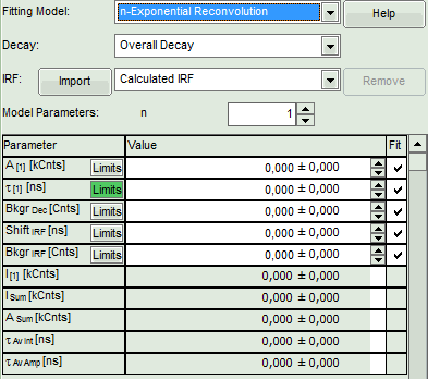
Lower left: Lifetime fitting parameters. Here lifetime fitting models can be defined. Fitting is then applied to the lifetime graph(s) on the lower center (TCSPC histogram).
Lower center/left: By default, this set shows the TCSPC histogram of all photons in the image in green (= dataset 0) and the TCSPC histogram of a single pixel in grey (= dataset 1). In red an estimation of the instrument response function (=IRF) is shown. The IRF reconstruction is deducted from the rising edge of the TCSPC histogram.
- To enhance the lifetime contrast within the daisy pollen, adapt the color scale from 0.7 to 2 ns by typing these values as limits for the Fast Lifetime color scale.
Note:
The default lifetime scale stretches from -0.5 to 41.6 ns. The physically impossible value of -0.5 ns is explained by the fact, that SymPhoTime places the 0 value at the rising edge of the decay in the TCSPC window. As a mean arrival time is calculated, it is possible that in dark regions only one or two photons caused dark count noise are detected which are randomly detected before the laser pulse in the TCSPC window.
Reasonable limits can either be found by dragging the limit bars in the color scale “Fast Lifetime” histogram or by considering the peaks of the “Lifetime Histogram”. Entering fixed values has the advantage that different images can be compared later.
Response:
The color scale in the image adapts and lifetime contrasts in the pollen become visible.
Determine start parameters for fitting
- In the fitting parameter table, change the fitting model to “n-Exponential Reconvolution Fit”.
Response:
- In the TCSPC window, the IRF is displayed in bright red, the data fitting limits are moved to the border of the TCSPC window.
- The new fitting parameters “Shift IRF” and “Bkgr IRF” (=background IRF) appear in the fitting parameter table.
Note:
The software offers the possibility to fit the data using a n-exponential tailfit or a n-exponential reconvolution fit. A tailfit can be used when the fitted lifetimes are significantly longer than the instrument response function. A reconvolution fit is usually preferable, because the complete decay is fitted, while for a tailfit, the start of the fitting range is usually a bit arbitrary.
For explanation about the fitting model and the used equations, click on the “Help” button next to the selected model. This opens a help window containing the fitting equation and the explanation of the different parameters.
- Click “Initial Fit” (marked in orange).
Response:
- A single exponential reconvolution fit is performed. In the TCSPC window, the fit is displayed as a black line. Below, the residuals (= raw data fit values) are displayed.
- Fit values appear in the fitting table.
Note:
Usually, a decent fit is characterized by the following criteria:
The fitted curve overlays well with the decay curve. In the residual window, the values spread randomly around 0.
The χ²-value approaches 1.
The calculated fitting values are reasonable.
Usually the fitting model with least parameters is selected.
In this example it is obvious that the applied single exponential reconvolution fit is not suited to fit the decay curve.
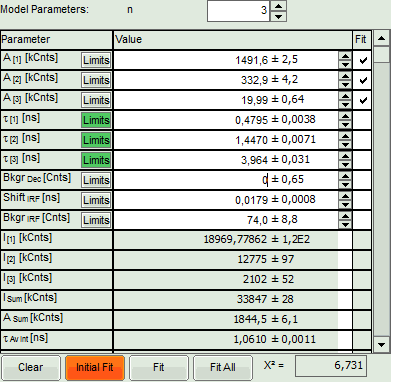
- Increase the “Model Parameters” to n = 2.
- Again, click on “Initial fit”.
Response:
The fit quality increases, but still the fit quality is not sufficient.
- Increase the “Model Parameters” to n = 3.
- Again, click on “Initial fit”.
Response:
The fit quality increases, but still the fit quality is not sufficient.
Note:
In spite of this, in this tutorial we will assume that the result was satisfactory. The autofluorescence and staining of the daisy pollen result in a complicated pattern, and the resolution of the pattern is not the scope of this tutorial, which just wants to explain the function of the analysis. The fit mainly differs from the data in the region around the instrument response function.
- For fitting of a 3-exponential decay into every pixel, a certain number of photons is necessary. How many, is determined by the complexity of the model. In order to check whether the photon number is sufficient for the model suggested, click on an average pixel of interest in the FLIM image.
Response:
The corresponding decay is updated in grey in the graph.

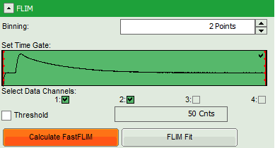
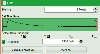
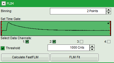
- In this case, the pixel decay contains less than 100 photons in the maximum, which makes it improbable that is can be easily fitted with a 3-exponential model. Therefore, perform a pixel binning by increasing the “Binning” to two points and click “Calculate FastFLIM”.
Response:
The image is recalculated, but now, 2×2 pixels are binned to 1, thereby increasing the number of photons per pixel 4fold, while sacrificing optical resolution.
- Click again on a similar pixel in the image as before and see how the decay has become higher.
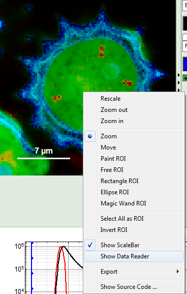
- Place the cursor over the image, activate the context menu with a right mouse click and select “Show Data Reader”.
- Move the mouse around the image and read the photon numbers. Inside the pollen, there are about 5000 - 7000 counts, outside the pollen the image intensity is below 100.
- Therefore, we activate the “Threshold” and enter a threshold number of 1000.
Note:
The threshold determines, which pixels are fitted with the lifetime model and which are not. As the area around the pollen is not important for the analysis, we can exclude those pixels from the analysis. This also decreases the processing time.
Perform a FLIM Fit
- In order to increase the fitting quality, we make a few assumptions:
- We assume that the excitation pulse does not shift within the image acquisition time within the TCSPC window, therefore we fix the parameters “Shift IRF” and “Bkgr IRF”. This is practically always valid. In case of an IRF estimated from the decay like here, these parameters can also be set to 0, as the IRF was derived from the decay.
- As we can see from the pixel decay in grey, the background before and after the decay is practically 0.Therefore, we can also fix this parameter “Bkgr Dec”to 0. This is also very often valid.
- Third we fix the three fitted lifetimes. If the sample contains only three fluorophores, this is also a valid approach, as long as the lifetime of the components does not depend on the local environment within the sample.
Note:
The aim of this procedure is to minimize the number of variable parameters, as every variable parameter also adds noise to the fit. It depends on the sample, to which extend this can be done.
- Do NOT click “Initial Fit” or “Fit” at this stage!
- Click “FLIM Fit” in the upper panel.
Response:
A 3-exponential reconvolution fit is performed on each pixel. The result is:
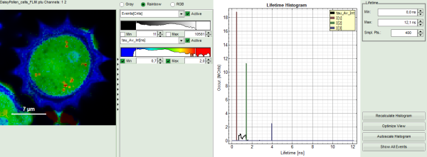
- An updated FLIM image. The colors can slightly change, as now the calculated intensity weighted average lifetime “tau_Av_Int” is displayed, in contrast to the “Fast Lifetime”, which is just the mean arrival time and contains e.g. background photons.
- An updated lifetime frequency histogram on the upper right. The fixed individual lifetime components are displayed as vertical bars.
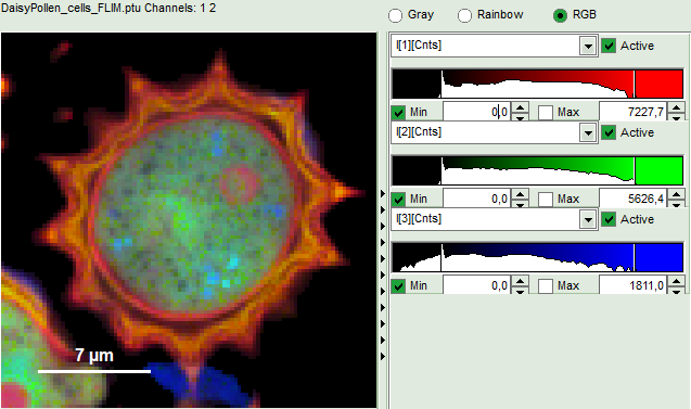
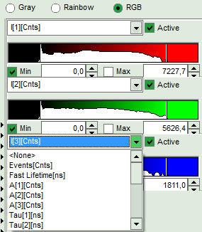
- The three lifetime components can be displayed in a false color scale. Therefore switch the display to “RGB” and adapt the intensities of each color as preferred.
Note:
I[1], I[2], I[3] correspond to τ[1], τ[2], τ[3], respectively in the TCSPC fitting panel. It is also possible to plot the amplitudes instead of the intensities or to switch off individual components.
- When the desired view is set, click “Save Result”.
Response:
A result file (“FLIM.pqres”) is stored under the raw data file (DaisyPollen_FLIM.ptu).
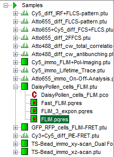
- Later, clicking on the result file reopens the file in the same way as it was stored.
