This is an old revision of the document!
~~TOC~~
SymPhoTime 64 Analysis Tips and Tricks
Summary
This tutorial explains a few features of SymPhoTime64 that can help to make working with the software more comfortable. In detail, this tutorial covers:
- Different file-types used or generated by SymPhoTime64
- Image Display
- ROI-handling
- Export options
This tutorial assumes SymPhoTime V2.0
General UI Philosophy
- right clicking on graphs/images gives additional options and tools otherwise hidden
File-Type Overview
| Workspace: may contain these Filetypes | Content of the file | How to get such a file in the workspace | How to open/process |
|---|---|---|---|
.ptu | Raw data in a unified TTTR-format |
|
|
.pqres | Result file |
|
|
.pck | internal file |
| this file type is for software internal purposes only, so the user does not need to use it. |
.pco | Comment file, contains manually entered text (e.g. information about the experiment) | Menu: File → Create Comment | Double Click |
.bmp | Contains a camera image | Save a camera image generated by the fluorescence or back reflection camera (only MT200 - users) | Double Click |
Working with the different file types
Raw data (''.ptu'') files
- double click on any
.ptu(raw data) file opens a file viewer, in which you find information about the file type and acquisition settings
 Fig. 1: ''.ptu'' file information and comment
The general file information contains for example:
- the number of pixels
- the image size (if the image has been acquired with a scanner controlled by the SymPhoTime software or the size info has been entered before the measurement, either manually in the “Acquisition” - tab or automatically for remotely controlled FLIM-imaging
- the imaging mode (mono- or bidirectional)
- whether it's a t2 or t3 type file
- Info that was entered into the text field during the acquisition (you cannot change this information after the acquisition)
More detailed information can be found in the “Header” - tab:

Comment (''.pco'') files
- To read or edit a comment-file (
.pco), just double click it.
Contrary to the comment entered prior the start of the measurement, the comment file can be edited at any time.
The comment entered before the measurement is stored directly inside the .ptu file and cannot be modified after the measurement (see figure 1).
Result (''pqres'') files
- Double clicking a
.pqres(result) file opens the result of a particular analysis script.
Result files also contain a comment which can be displayed via the file menu: File → Show Comment.

Typically the result-file opens with a preview display (Image, FCS-traces, TCSPC-curve or Time Trace - depending on the type of analysis). Additionally the “Comment” - tab of an online-analysis will contain relevant information about the measurement. To check the values calculated during an online analysis, select the “Comment”-tab.
The kind and amount of the information of course depends on the type of online analysis:
Image
 Fig. 2: Comment Tab of an imaging online analysis result
 Fig. 3: Images Tab of an imaging online analysis result
- Max. Photons (in the brightest pixel for the selected data channel)
- Max. Countrate (calculated taking into account the pixel recording times)
- Avg. Photons (in a pixel)
- Avg. Countrate (calculated taking into account the pixel recording times)
- Frames (especially important for LSM upgrade kits where in general several frames are recorded, while for an image acquired with the MicroTime, the image consists of a single frame)
FCS (for each of the max.2 data channels)
 Fig. 4: Comment Tab of an FCS online analysis result
 Fig. 5: Curves Tab of an FCS online analysis result
- Max. Countrate
- Avg. Countrate
- G(0)
- Num. Molecules (calculated from the average countrate and G(0))
- mol. Brightness (in kcps/s/molec.)
- if 2 data channels are active, also G(0) of the crosscorrelation is calculated.
Time-Trace
- Max. Counts
- Av. Counts
TCSPC
- Max. Counts (number of photons in the peak TCSPC-channel)
You can also add additional information and save this using the “Save Comment” - button. The modified comment is stored in the same (.pqres) file.
Image Display
- Images can be drawn in 3 ways (for this, open the file
FLIM_3_expon.pqres, associated to the raw data fileDaisyPollen_cells_FLIM.ptu) - toggling between the different display options can be done by selecting the desired display option above the scale.
| Grey Scale | Rainbow Scale | RGB Scale |
|---|---|---|
 |  |  |
1 selectable parameter encoded:
| 2 selectable parameters encoded as:
| 3 selectable parameters encoded as:
|
- some parameters are only available after performing a FLIM-Fit (i.e. the different lifetime components and amplitudes
- to adjust the scale, you can either
- type the min and max-value
- place the cursor above the scale, right click and select “Scale (ALL)“.
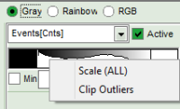 This adjusts the minimum to the minimum value of this parameter in the image. This may also mean that if there a a few pixels with extreme values, e.g. very long lifetimes of some background pixels, that the contrast within the structures of the image is not as clearly visible anymore. On the other hand, as the min and max values are then display as scale limits, you can get an easy idea of the parameter range in the image.
 - place the cursor above the scale, right click and select “Clip Outliners”. This feature ignores outliners of the parameter (i.e. the 5% lowest and highest values).

- when looking at the Fast Lifetime parameter, in the unbinned image, which calculates the mean of the photon arrival times, you will notice that the lifetime values have partially negative values:


- this happens, as the rising edge of the decay is chosen as 0. Background pixels with just a single photon which might be before this pixel can therefore have negative Fast Lifetime values.
- in fitted images, constraints can be set (e.g. 0 as minimum lifetime) in the TCSPC fitting panel
- the fast lifetime in an ideal system should equal the intensity weighted average lifetime [τ av. int.]. Usually, fitted lifetimes tend to be slightly shorter, as the background photons are excluded from the calculation.
- In images obtained with PIE-excitation, the fast lifetimes are usually meaningless, as in this case the photons from 2 decays are taken into account.
Color Smoothing
- In a “Rainbow Scale Image”, a color smoothing can be introduced. When checking “Smooting” below the intensity axis, a width defined can be defined for a Gaussian distribution which is overlaid to the image and used to improve the optical appearance of the image. As in many cases the pixel size in the image is smaller than the optical resolution, taking into account the neighbouring pixels is also a valid approach to de-noise the image.
- The smoothing is only applied to the parameter encoding the color scale. Take a look at the effect in the following example from the
Fast_FLIM.pqresfile which is associated to the fileDaisyPollen_cells_FLIM.ptu
 Fig. 6: No Smoothing
 Fig. 7: Smoothing = 100nm
 Fig. 8: Smoothing = 200nm
 Fig. 9: Smoothing = 400nm
- As can be seen for this example, moderate smoothing can despeckle the image slightly, while high smoothing can completely mask certain features and therefore also introduce artifacts. Therefore please handle the tool with care
- NOTE: As the smoothing is just a display function that does not affect the raw data, smoothed images can be exported as
.bmp, but not as ASCII or.tif, and also the smoothing does not affect the lifetime histogram - Take care that you record the data with the correct physical dimensions. While in images taken with the MT200 this is done automatically, in LSM upgrade systems, which are not remotely controlled by the LSM software via a handshake, the image size is not known unless typed in before the acquisition (see online tutorials about FLIM and FLIM-FRET imaging)
Working with ROIs
Selecting ROIs
In Images, ROIs can be selected using the context menu (Right Click):

- you can mark several areas with the same or different selection tools by keeping the
<Shift>key pressed while drawing the different ROIs - if you want to remove some of the pixels from the ROI selection, just keep the
<CTRL>- key pressed when using a ROI selection tool to unselect unneeded pixels from the selection. - If you want to start from scretch again, select “Select all as ROI”
- you can also invert the selection using “Invert ROI”
The following ROI-selection tools are available:
Paint ROI
 Marks the pixels the mouse passes over. The faster the mouse pointer moves, the broader is the marked line of pixels
Free ROI
 draw a free shape, the pixels within the drawn shape selected
Rectangle ROI

Ellipse ROI

Magic Wand ROI
 marks areas with a similar fast lifetime
Undo ROI selection
Using <CTRL>+<Z> you can undo a selection (you can also redo by pressing <CTRL>+<Shift>+<Z>), as shown in this example:
| 1. Start image, in this case the daisy-pollen image from the demo workspace, we choose the “FLIM_3_expon.pqres”. The task is to define a ROI from the blue area below the pollen for this illustration example. |  |
| 2. Select a ROI (in this case, the free ROI-tool is used) |  |
| 3. To mark the other part of the blue area, keep the <Shift> - key pressed while marking the second area. For illustration, also some orange parts where marked. |  |
4. Press <CTRL>+<Z> to undo the second selection. | |
| 5. Mark the second region again, keeping the <Shift> - key pressed. |  |
Example: marking several spots with a similar lifetime:
1. Click on the file FAST_FLIM.pqres, which is associated to the file DaisyPollen_cells_FLIM.ptu |  |
| 2. first mark one structure with the magic wand tool. All other pixels turn grey, therefore it is not possible anymore to know which pixels to select. |  |
| 3. Therefore invert the ROI |  |
| 4. then keep the <CRTL>-button pressed and click on the other areas with a long lifetime (it is also possible to change the ROI-selection tool). |  |
| 5. now invert the ROI again, and you have marked all similar areas within the Pollen. |  |
How to use the magic wand tool
The magic wand tool marks region with a similar lifetime range. “Similar” in this sense is an arbitrary definition, but the sensitivity “Magic Wand Thres.” of the magic wand tool can be adjusted in a box below the intensity and color scaling options (see in the screenshots below). Adjusting the Magic Wand Threshold can help to easier mark objects in the image as shown in the example:
 Thresh. = 10 (default value) |  Thresh. = 20 |  Thresh. = 30 |  Thresh. = 40 |
The magic wand tool is based on the displayed image, therefore the sensitivity of the selection is also dependent on the scaling of the color-encoded component (in general, the lifetime). Changing the color scale can also change the sensitivity of the tool as shown in this example:
 Magic Wand selection ⇓  |  Magic Wand selection ⇓  |
How to get values of a parameter along a line
In SymPhoTime 64 there is the option to get the Intensity profile along a line from the GUI element “slice direction” in the following GUIs

- FLIM
- Pattern Matching
- Fast Pattern Matching
- Focal Width
- Gated STED Image
- Confocal + STED Image
In Analysis GUIs “FLIM” and “Pattern Matching” the feature is made availble upon clicking on the “Resolution estimation” tab. 
or

Let us take as an example the “FLIM Analysis” GUI
| Rectangular | Upon left mouse clicking on any point of the image the intensity profle is plotted along the X- and Y axis of the image  |
| Diagonal | Having the mouse left button continuously pressed draw a line in the image.  |
Now use the drop-down list to select the parameter used for the “gray-scale” and select “FastLT” (or any other parameter of your choice)
 .
.
Then you get the corresponding gray level image according to “FastLT” and by clicking on the selected line the graph in the lower panel is updated and the now the profile of the the “FastLT” along the line is displayed.

Note: The title and units of the Y axis of the graph will not be updated.
Rescaling of the lower graph might be necessary
As a final step you can right click on the graph and export the line profile data.
Export Options
Export of graphs and images can usually be done via the context menu via a right mouse click with the mouse being over the image or graph. Some scripts also have defined export buttons in the control panel on the left.
Images
For images, there are the following export options (right clicking on any displayed image will show the export dialogue:

Formats
Bitmap

- The image is exported as shown on the screen.
- The color scale is not exported
- If the image size on the screen is increased (e.g. by iding the script-tab), the scale bar may adapt.
- The scale bar can be hidden by unchecking “show scale bar” in the context menu
Bitmap with Color Scale

- The image is exported as shown on the screen.
- The intensity and/or color scale is exported
- If the image size on the screen is increased (e.g. by iding the script-tab), the scale bar may adapt.
- The scale bar can be hidden by unchecking “show scale bar” in the context menu
1 to 1 Bitmap

- Every pixel in the image is exported as one single pixel in the bitmap
- The color scale is not exported
- changes in the intensity scale are adapted to the image
ASCII

- the file is exported as a text file
- Every plotted parameter is saved as an array in the text file, before every array, there's a small header that indicates dimensions and the shown parameter.
Thus depending on the plot type, the file contain several arrays:- greyscale images : 1 array, i.e. intensity
- rainbow images: 2 arrays, i.e. intensity + fast lifetime
- RGB images: 3 arrays, i.e. amplitude 1-3
- for importing into processing programs as ImageJ, best export each parameter as greyscale image, delete the header lines and import as text image into ImageJ. Make sure that the decimals number have the same country settings in both programs to avoid import problems.
TIFF

- Every pixel in the image is exported as one single pixel in the tiff
- the tiff format for the number is float, therefore the real values can be displayed.
- Each parameter is stored as different greyscale-frame, therefore export of an RGB-image results in a tif-image stack with 3 layers
- As absolute values are exported, the displayed intensity scale is not relevant
- The image size is exported as well, however the current ImageJ always shows cm.
You can manually set it to µm via: Image Properties → Unit of Length → µm.
Clipboard
- This feature exports the image as in the bitmap-option, but into the clipboard.
The image can than be pasted into a graph or text program (e.g. word document) via<CTRL>+<V>
Binary
- This export option is not found in the context menu, but in the FLIM-script and a few others as a separate button.
- It exports the image as a
.bin-file, which can be imported e.g. into phasor analysis software and is also supported by the open microscopy platform. - TCSPC-binning is applied to the export of these images.
Graphs
- for graphs, e.g. the TCSPC-Decay plot in the FLIM-script, can be exported in an ASCII-format as well as in a bitmap format. If the graphs consists on different cells, e.g. the decay and the residuals as shown, it is possible to select, which cells should be exported.

Export ASCII selected cell

- the active cell is the cell below the mouse pointer, the color of the lines in the active cell change to green.
- The active cell in this example is the TCSPC decay window, exporting the active cell just exports the decays in the upper window without the residuals
- the exported file is a text file that can be loaded into Excel or other programs.
Export ASCII visible cells

- all open cells are exported in this option, i.e. if the graph is plotted as shown above, the decays and the residuals are exported.
- If the residual cell is closed by clicking on the small green “-” on the upper left corner of each cell (see below), the active cell equals the visible cell, and the export result is the same as exporting just the active frame
- the exported file is a text file that can be loaded into Excel or other programs.
Export ASCII all cells
- all cells are exported. In our example, TCSPC-decays and residuals are both exported, independent from whether the all cells are open or not.
Export bitmap

- the graph is exported as plotted bitmap.
Copy to clipboard
- the graph is exported as an image to the clipboard as plotted and can be pasted into a graphic program or e.g. a word document via
<CTRL>+<V> - In contrast to the bitmap-export, a highlighted cell in the the clipboard-copy remains highlighted. If this is not wanted, just move the mouse slightly out of the cell before exporting to clipboard
Fitting Results
- For *Fitting Results*, e.g. Lifetime-Fits, the values can be exported as an ASCII-table either into a file or the clipboard, from where it can be directly pasted into e.g. Excel or a similar program. To export, you can use either the context menu, as with graphs and images, or the icons above the fitting panel.

- The feature can not only export the fitted values of one curve, but also be applied for the fits of several curves simultneously. To illustrate this, mark several ROIs in the image, as illustrated in the image below:

- click on “initial fit” to get resonable staritng parameters, then “fit all”
- When data are exported now, the fitting values of each fitted data set are stored in an additional line

- If you want to view all the fitting parameters in one window, you can just click on “Show all” on the upper left , and a window opens, which displays all fitting parameters side by side.


- Exporting from this window exports also all fitting values.
- In an analogous fashion, also FCS-fitting data can be exported.