ROI Fitting Using the FLIM Analysis
Summary
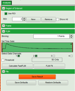
This tutorial shows step-by-step, how the FLIM script of SymPhoTime 64 can be used to fit several regions of interest (ROIs), and how to extract and interpret the results. In details, the FLIM script is started using a daisy pollen image from the “Samples” – workspace, then three regions of interest are defined which are finally fitted.
Step-by-Step
Select a file and start the script
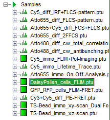
- Start SymPhoTime 64 software.
- Open the “Samples” workspace via “File\open Workspace” from the main menu.
Note: The “Samples” workspace is delivered with the SymPhoTime 64 and on the CD-ROM drive and contains example data to show the function of the SymPhoTime data analysis. If you haven't installed it on your computer, copy it from the DVD onto a local drive before going through this tutorial.
Response: The files of the sample workspace are displayed in the workspace panel on the left side of the main window.
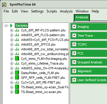
- Highlight the file
DaisyPollen_cells_FLIM.ptuby a single mouse click.
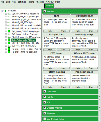
- Select the “Analysis”-tab and in there, open the drop down menu “Imaging”.
Note: The drop down menu can be opened and closed by clicking on the grey button on the left side of the header of the drop down menu: 
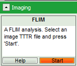
- Start the FLIM script by clicking on “Start”.
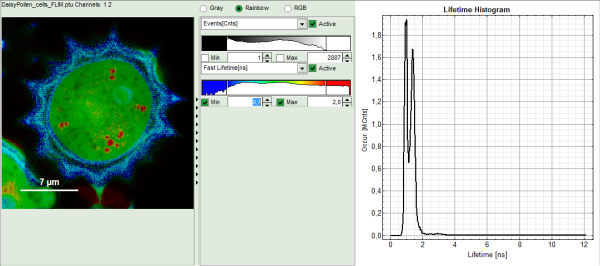
Response: The FLIM script is applied to the file DaisyPollen_cells_FLIM.ptu. Thereby, a new Window opens:
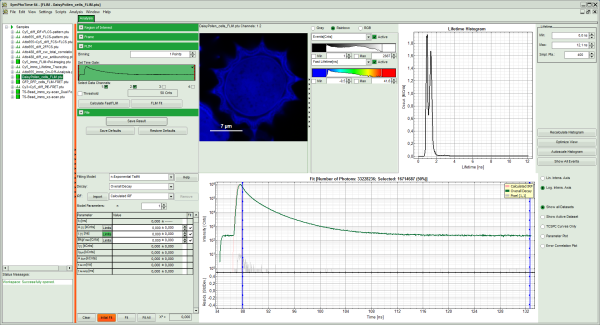
Note: The window contains five different regions:
- Upper left: imaging analysis options.
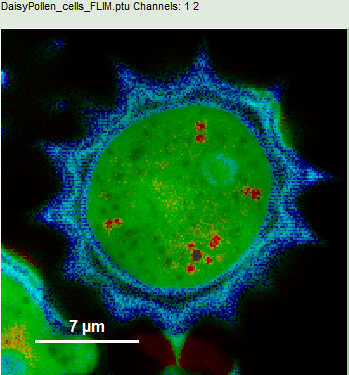
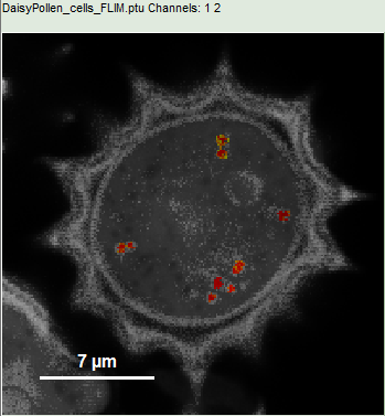
- Upper center: Fast FLIM image, displayed in false color scale. The brightness encodes the intensity while the color encodes the average “Fast FLIM” lifetime, i.e. the mean arrival times of the photons after the laser pulse. When not defined otherwise, intensity and color scale stretch from minimum to maximum. As the mean arrival time of the background photons in the areas where no fluorescence is detected, is randomly spread over the TCSPC window, the mean photon arrival time of the dark background is usually very long (up to 1/2 of the TCSPC window), which makes the color scale loaded by default sometimes unsuited for displaying the lifetime contrast in the actual sample. In this case, the scale has to be adapted.
- Upper right: Fluorescence Lifetime Histogram. Here the frequency of photon counts corresponding to the individual mean lifetimes is plotted. The settings of the plot can be adapted using the controls on the right of the plot.
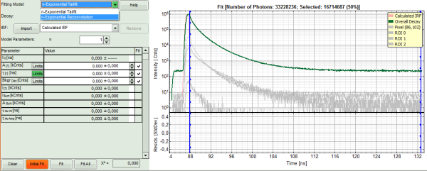
- Lower left: Lifetime fitting parameters. Here lifetime fitting models can be defined. Fitting is then applied to the lifetime graph(s) on the lower center (TCSPC histogram).
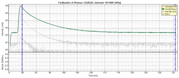
- Lower center/left: By default, this set shows the TCSPC histogram of all photons in the image in green (= dataset 0) and the TCSPC histogram of a single pixel in grey (= dataset 1). In red an estimation of the instrument response function (=IRF) is shown. The IRF reconstruction is deducted from the rising edge of the images TCSPC histogram.
- To enhance the lifetime contrast within the daisy pollen, adapt the color scale from 0.7 to 2 ns by typing these values as limits for the Fast Lifetime color scale.
Note: The default lifetime scale stretches from -0.5 to 41.6 ns. The physically impossible value of -0.5 ns is explained by the fact, that SymPhoTime places the 0 value at the rising edge of the decay in the TCSPC window. As a mean arrival time is calculated, it is possible that in dark regions only one or two photons caused dark count noise are detected which are randomly detected before the laser pulse in the TCSPC window.
Reasonable limits can either be found by dragging the limit bars in the color scale “Fast Lifetime” histogram or by considering the peaks of the “Lifetime Histogram”. Entering fixed values has the advantage that different images can be compared later.
Response: The color scale in the image adapts and lifetime contrasts in the pollen become visible.
Select 3 Regions of Interest (ROI)
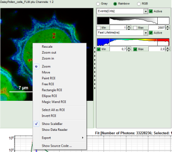
- Keep the mouse pointer over the image and open the context menu by a right mouse click.
- Select a ROI tool in the context menu, e.g. the “FreeROI” tool.
Note: The different ROI tools are used in the following way:
Paint ROI: highlights the pixels the mouse cursor is guided over while the left mouse button is activated. The faster the cursor is moved the broader is the area of pixels highlighted around the mouse.
Free ROI: moving while keeping the left mouse button activated marks the area within the drawn shape.
Rectangle ROI: to draw rectangular ROIs.
Ellipse ROI: to draw elliptic ROIs.
Magic Wand ROI: when activated, clicking activates all neighboring pixels with a similar Fast Lifetime. Especially useful for marking spotted structures.
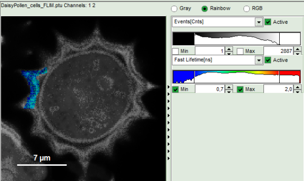
- Draw a ROI in the blue rim of the pollen by maintaining the left mouse button activated while circling the selected part of the image as shown:
Response:
- Everything except the circled area is displayed only in grey scale.
- In the lower part of the window, a new decay appears in grey, which contains the photons from the selected pixels. This new decay is labeled “ROI 0”.
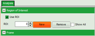
- On the upper left, open the drop down menu “Region of Interest” and click on “New”.
Response:
- In the “Region of Interest” drop down, the ROI number is set to “1”.
- The whole image is displayed in color scale again.
- In the decay legend, ROI 1 is added.
- As ROI 1 contains still all photons of the image and equals the “Overall decay”, no new curve is displayed.
- Place the cursor over the image, select in the context menu (right mouse click) the “Rectangle ROI” and mark a rectangular ROI in the green central part of the pollen.
Response:
- Everything except the marked area is displayed only in grey scale.
- In the lower part of the window, a new decay appears in grey, which contains the photons from the selected pixels. This new decay corresponds to “ROI 1”.
- Mark a third ROI. Therefore, on the upper left, open the drop down menu “Region of Interest” and click on “New”.
Response:
- In the “Region of Interest” drop down, the ROI number is set to “2”.
- The whole image is displayed in color scale again.
- In the decay legend, ROI 2 is added.
- Place the cursor over the image, select in the context menu (right mouse click) the “Magic Wand ROI” and click on a red region in the pollen.
Response:
- Everything except the marked area is displayed only in grey scale.
- In the lower part of the window, a new decay appears in grey, which contains the photons from the selected pixels. This new decay corresponds to “ROI 2”.
Note: The new decay wich stems from the last and smaller ROI contains considerably less photons. Ideally, decays selected for ROI fitting should contain ~10000 – 50000 photons in the peak.
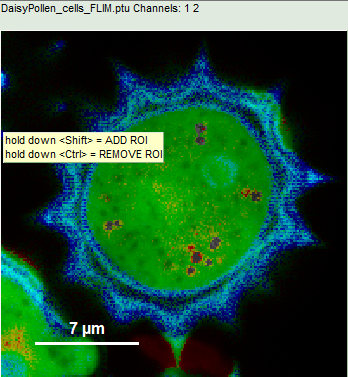
- As the decay contains much less photons than the other ROIs, we add other regions to the same ROI. In order to recognize the red regions, go to the context menu and select “Invert ROI”:
Response:
- Everything except the originally selected pixels for ROI 2 are displayed in color scale.
- Keep the <CRTL>-button pressed while clicking on the other red dots in the image. With every selection, the corresponding red dot is greyed out.
- Again, select “Invert ROI” in the context menu.
Response: Now only the red dots of the pollen image are highlighted, everything else is greyed out. The decay corresponding to ROI 2 contains now the photons from all marked dots.
Note:
To review the different regions, go to the drop down menu “Regions of Interest” and change the number between 0 and 2. The image will display the corresponding image with the selected ROI.
To export the images with a marked ROI, keep the cursor over the image with the selected ROI, open the context menu with a right mouse click and select one of the export options:
Bitmap exports the image as a bmp file. If the scale bar is displayed, the image including the scale bar is exported.
Bitmap with color scale exports the image as a bmp file including the intensity and color scale next to the image.
1×1 bitmap exports the image as a bmp file with one pixel of the image being exported as one pixel in the image file. In the other bitmap export options, the image is exported as displayed.
ASCII exports the image as ASCII array using a text file format. Thereby one array encodes the intensity values, while a second array encodes the Fast Lifetime values. After removal of the header and the unwanted array, individual arrays can be imported in graphic programs, e.g. ImageJ as a text image. These images contain the full count resolution of the raw image.
Perform a Lifetime Fit on the Selected Regions (ROIs)
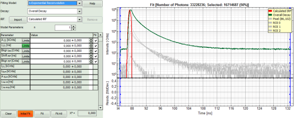
- In the decay form on the lower left, select n-exponential reconvolution as fitting model.
Response:
- In the TCSPC window, the IRF is displayed in bright red, the data fitting limits are moved to the border of the TCSPC window.
- The new fitting parameters “Shift IRF” and “Bkgr IRF” (=background IRF) appear in the fitting parameter table.
Note: The software offers the possibility to fit the data using a n-exponential tailfit or a n-exponential reconvolution fit. A tailfit can be used when the fitted lifetimes are significantly longer than the instrument response function. A reconvolution fit is usually preferable, because the complete decay is fitted, while for a tailfit, the start of the fitting range is usually a bit arbitrary.
For explanation about the fitting model and the used equations, click on the “Help” button next to the selected model. This opens a help window containing the fitting equation and the explanation of the different parameters.
- Under “Decay” select “ROI 0”.
Response:
- The TCSPC curve of ROI 0 is highlighted in green.
- Click: “Initial Fit” (marked in orange).
Response:
- In the TCSPC window, the fit of ROI 0 is displayed as a black line. Below, the residuals (= raw data fit values) are displayed.
- Fit values appear in the fitting table.
Note: Usually, a decent fit is characterized by the following criteria:
The fitted curve overlays well with the decay curve. In the residual window, the values spread randomly around 0.
The χ²-value approaches 1.
The calculated fitting values are reasonable.
Usually the fitting model with least parameters is selected.
In this example it is obvious that the applied single exponential reconvolution fit is not suited to fit the decay curve.
- Increase the “Model Parameters” to n = 2.
- Again, click on “Initial fit”:
Response:
- The fit quality increases, but still the fit quality is not sufficient.
- Increase the “Model Parameters” to n = 3.
- Again, click on “Initial fit”.
Response:
- Now a good fit result is achieved.
- To check whether this is really the best possible fit, increase the “Model Parameters” to n = 4.
- Again, click on “Initial fit”.
Response:
- The fit becomes even slightly better, but looking at the fitting parameters, we find an amplitude A4 with a negative value “-40”. This is not expected, and not physically logical. Therefore, this decay is best described by a 3-exponential model.
- Decrease the “Model Parameters” to n = 3.
- Again, click on “Initial fit”.
Response:
- Now a good fit is achieved.
- To compare the fit with other ROIs, we select: “Fit all”.
Response:
- Every decay is fitted with a 3-exponential fit.
- As the last fit is ROI 2, this curve is shown in green at the final window.
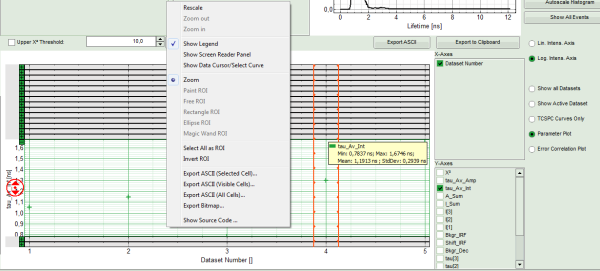
- To compare the fitting data, either toggle between the graphs by selecting as “Decay” ROI 0, ROI 1 or ROI 2 or click on “Parameter Plot” (right next to the TCSPC graph).
Response:
- Instead of the TCPSC curve, the fitted parameters appear in a graph.
- Select the parameter you would like to display (e.g. T_av_Int, the intensity-weighted average lifetime, which - neglecting background photons – roughly corresponds to the Fast Lifetime).
Note: On the x-axis, the dataset name is plotted. The order is the same as in the decay menu:
1 = Overall decay, generated from all photons of the image.
2 = Pixel decay, including the photons from the last selected pixel.
3 = ROI 0
4 = ROI 1
5 = ROI 2
- Keep the cursor over the graph, and after a right mouse click, select from the context menu the “Export ASCII (All Cells)” option.
Response: A window opens, asking for a file name to store the fitting values. The data are stored as a .dat file.
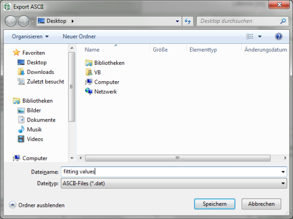
- The
.datfile contains the fitting values as table and can be opened e.g. using the Notepad program. They can also be imported into Excel or similar programs.
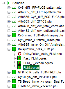
- Store the result file by selecting: “Save Results”.
Response:
- A result file (
FLIM.pqres) is stored under the raw data file (DaisyPollen_FLIM.ptu).
- Later, clicking on the result file reopens the file in the same way as it was stored.
Note:
This tutorial explains only a subset of the functions of the FLIM script. Also check the script explaining pixel fitting (Lifetime Fitting using the FLIM Analysis).
