FLIM-FRET Calculation for Multi Exponential Donors

This tutorial shows step-by-step, how the “Lifetime FRET Image” analysis of SymPhoTime 64 can be used to calculate pixel-by-pixel the average FRET efficiency in an image containing several cells transfected with Cerulean/YFP-constructs. To calculate the average FRET-efficiency, first the donor only lifetime is determined using cells that have only been transfected with the donor construct by performing a ROI-fit with the FLIM-analysis. The amplitude weighted average donor lifetime is used to calculate the average FRET-efficiency using the “Lifetime FRET Image” analysis.

FLIM-FRET is a robust method to determine the FRET efficiency of a suited donor acceptor pair. If the FRET-donor molecule has a more exponential decay kinetic, the amplitude weighted average lifetime has to be used to calculate the average FRET efficiency. The script usage is demonstrated on an image of several cells which have been transfected with CENP-B-Cerulean and YFP-CENP-A. Cerulean is a CFP variant an frequently used as a FRET donor. The CENP-complex consists on several proteins and is involved in mitosis. For further details on the sample, see S. Orthaus et al., Chembiochem. 2008, 9, 77-92, and the PicoQuant application note http://www.picoquant.com/images/uploads/page/ files/7267/appnote_flim_fret.pdf. The example image used is an image showing four cells, two of them only transfected with the CENP-B-Cerulean complex, the other two transfected with both constructs. Therefore, the same image can be used to determine the donor only lifetime and also to perform the pixel-by-pixel fit to calculate the FRET efficiency.

Note: This Step-by-Step tutorial was written for SymPhoTime version 2.5. There might be slight differences compared to other software versions. For example the way of setting an intensity threshold has changed. In the video the former version is shown.

• Start SymPhoTime 64 software.
• Open the “Samples” workspace via “File\open Workspace” from the main menu.

Note:
The “Samples” workspace is delivered with the SymPhoTime 64 and on the CD-ROM-drive and contains example data to show the function of the SymPhoTime data analysis. If you haven't installed it on your computer, copy it from the the DVD onto a local drive before going through this tutorial.

Response:
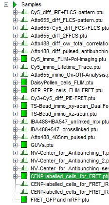
The files of the sample workspace are displayed in the workspace panel on the left side of the main window.

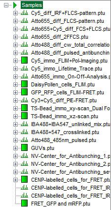
• Highlight the file CENP-labelled _cells_for_FRET.ptu by a single mouse click.

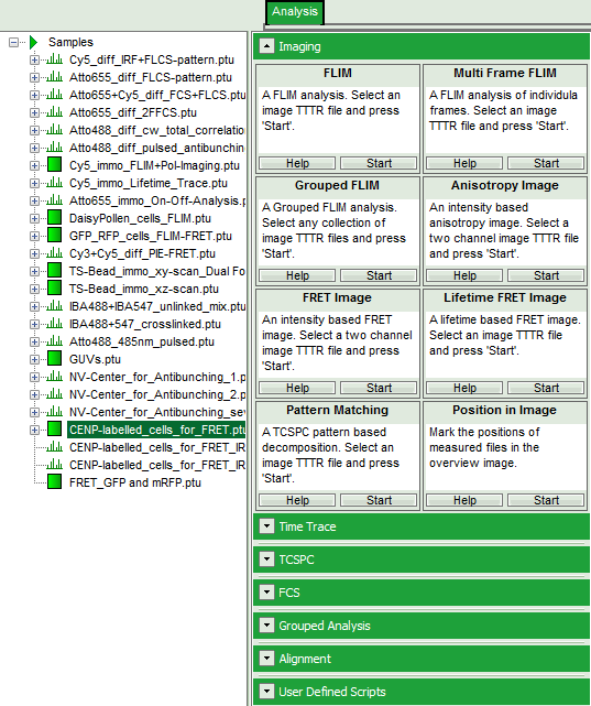
• Select the “Analysis” tab and in there, open the drop down menu “Imaging”.

Note:
The drop down menu can be opened and closed by clicking on the grey button on the left side of the header of the drop down menu:

• Start the FLIM script by clicking on “Start”.

Response:
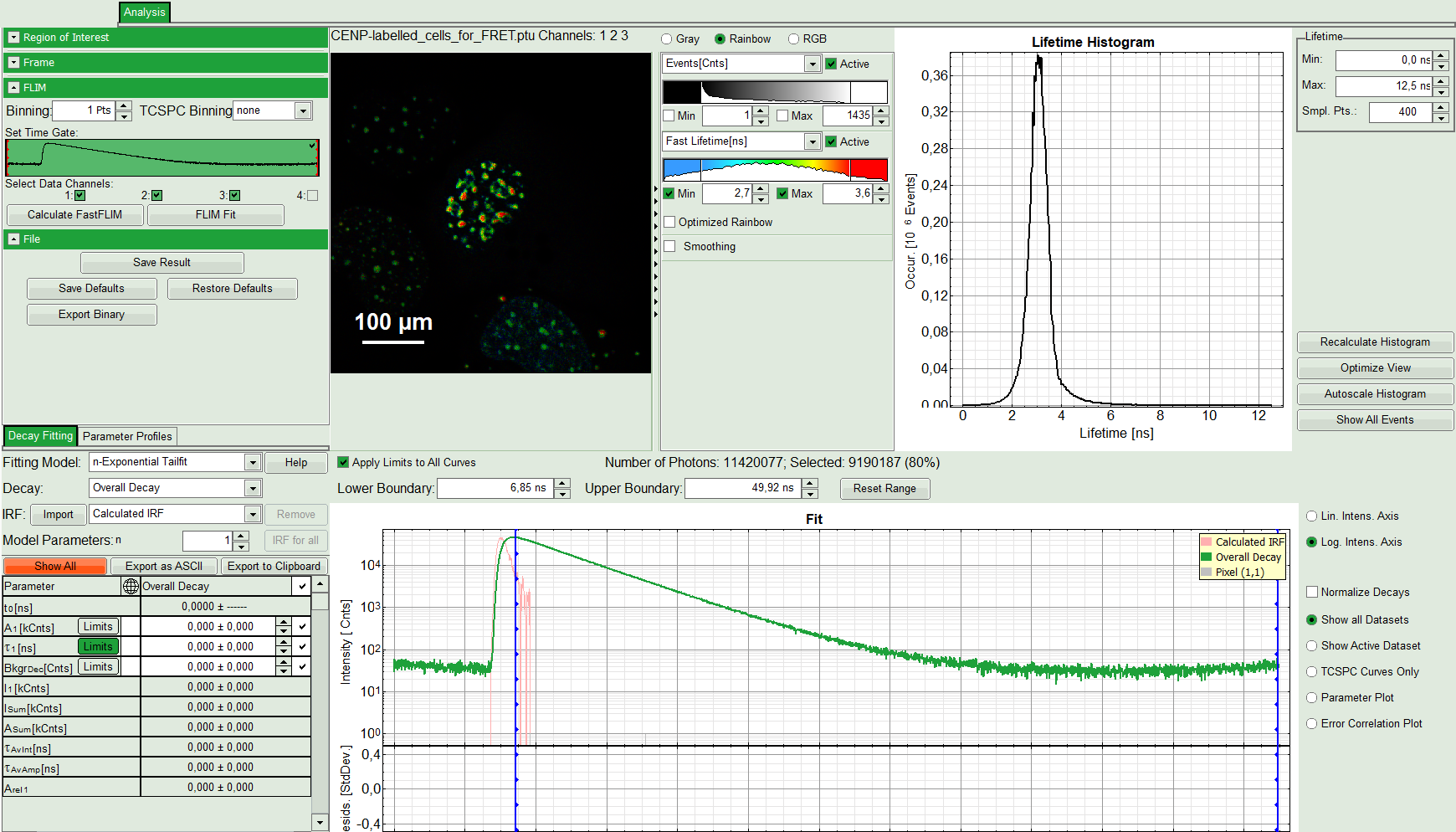
The FLIM script is applied to the file CENP-labelled_cells_for_FRET.ptu. Thereby, a new Window opens:

Note:
The window contains five different regions:
Upper left: Imaging analysis options.
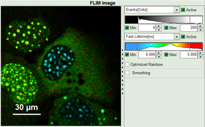
Upper center: Fast FLIM image, displayed in false color scale. The brightness encodes the intensity while the color encodes the average “Fast FLIM” lifetime, i.e. the mean arrival times of the photons after the laser pulse. When not defined otherwise, intensity and color scale stretch from minimum to maximum. As the mean arrival time of the background photons in the areas where no fluorescence is detected, is randomly spread over the TCSPC window, the mean photon arrival time of the dark background is usually very long (up to 1/2 of the TCSPC window), which makes the color scale loaded by default sometimes unsuited for displaying the lifetime contrast in the actual sample. In this case, the scale has to be adapted.
Upper right: Fluorescence Lifetime Histogram. Here the frequency of photon counts corresponding to the individual mean lifetimes is plotted. The settings of the plot can be adapted using the controls on the right of the plot.
Lower left: Lifetime fitting parameters. Here lifetime fitting models can be defined. Fitting is then applied to the lifetime graph(s) in the TCSPC histogram.
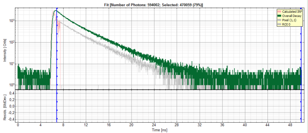
Lower center/left: By default, this set shows the TCSPC histogram of all photons in the image in green (= dataset 0) and the TCSPC histogram of a single pixel in grey (= dataset 1). In red an estimation of the instrument response function (=IRF) is shown. The IRF reconstruction is deducted from the rising edge of the TCSPC histogram.

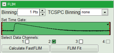
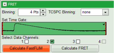
• As data channels, check only Channel 2, as in this channel the donor emission has been recorded.

• Press “Calculate Fast FLIM” to update the image.

Response:
The image and the graphs are recalculated, using photons only from channel 2.

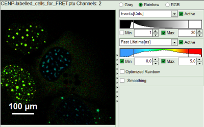
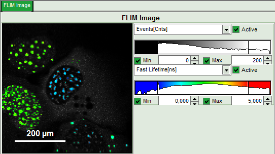
• To enhance the lifetime and intensity contrast, set in the image the intensity from 1 count to 30 counts and the lifetime from 0 to 5 ns.

Response:
The image scales are adapted.

Note:
Now four cells are visible, the two nuclei on the left have longer Fast lifetimes then the other two. These are the cells transfected only with the donor constructs.

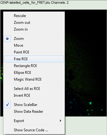
• Keep the mouse pointer over the image and open the context menu by a right mouse click. Select the “Free ROI” tool.

Note:
For more information about the different ROI selection tools, check the tutorial ROI fitting using the FLIM script.

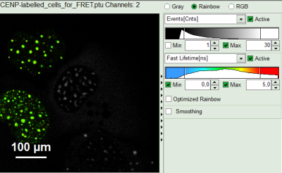
• Draw an ROI around one of the left cells by maintaining the left mouse button activated while circling the selected part of the image. Then release the left mouse button, press “Shift” continuously and cycle the other left nucleus. This way, the donor only cells are marked as ROI 0.

Response:

• Only the selected area is now shown in color.

• In the TCSPC window, the photons from ROI 0 are added in grey.

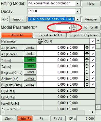
• In the decay form on the lower left, select n-exponential reconvolution as fitting model.

Response:

• In the TCSPC window, the IRF is displayed in bright red, the data fitting limits are moved to the border of the TCSPC window.
• The new fitting parameters “Shift IRF” and “Bkgr IRF” (=background IRF) appear in the fitting parameter table.

Note:
The software offers the possibility to fit the data using a n-exponential tailfit, a n-exponential reconvolution fit or a rapid reconvolution fit. A tailfit can be used when the fitted lifetimes are significantly longer than the instrument response function. Still a reconvolution fit is usually preferable, especially for FRET determinations, because the complete decay is fitted, while for a tailfit, the start of the fitting range is usually a bit arbitrary, and the short component can be underestimated. The rapid reconvolution model is used for systems with rapid reconvolution electronics (e.g. hybrid PMA-detector + MultiHarp photon counting board), where the peak count rates have been significantly higher than the pile up limit, or in cases, where the repetition rate has been too high to fit the decay completely into the TCSPC-window, e.g. 2PE excitation with 80MHz and dyes with a lifetime above ~3ns. For explanation on the fitting model and the used equations, click on the “Help” button next to the selected model. This opens a help window containing the fitting equation and the explanation of the different parameters.

• Under “Decay” select “ROI 0”.

Response:
The TCSPC curve of ROI 0 is highlighted in green.

• At the IRF, click on the “Import” button.

Response:
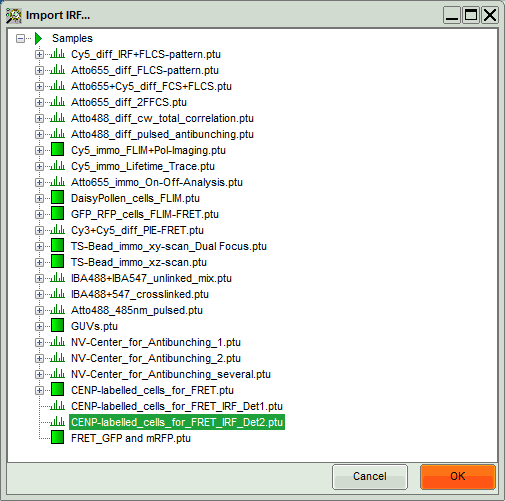
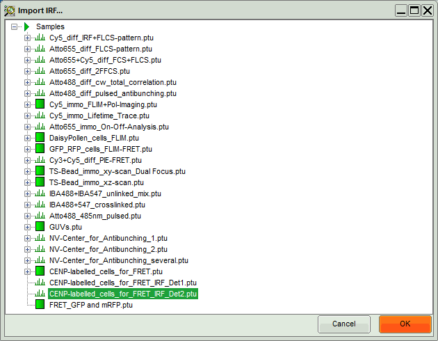
A window opens, where the file containing the IRF can be selected.

• Select the file CENP-labelled_cells_for_FRET_IRF_Det2.ptu and press “OK”.

Note:
This file contains a measured instrument response function (IRF) of detector 2. The best way to measure an instrument response function is measuring a dye that is highly quenched in a saturated solution of KI. See e.g. Szabelski et al., Appl. Spectrosc. 2009, 63, 363-368.

Response:
The decay of the imported IRF is shown in grey in the TCSPC window.

• Activate the imported IRF by selecting the IRF file in the IRF drop down menu.

Response:
The imported IRF is highlighted in red.

• As model parameters, select n=“2”.

Note:
In this case, the decay is double exponential. As it is not the scope of the tutorial to explain standard lifetime fitting (see the tutorial “ROI fitting using the FLIM script”), we skip the steps of finding the correct fitting model here.

• Click on “Initial Fit”.

Response:The fit is calculated.

• The software calculates the amplitude weighted average lifetime τ_{Av. Amp.}of 2.66. This is the result of the average donor lifetime in absence of FRET.

Note:
The fitted lifetime can slightly differ depending on the ROI drawn. It is important to use the amplitude weighted average lifetime. While the intensity weighted average lifetime corresponds to the real average arrival time of the photons and is therefore also close to the Fast lifetime in case of low background noise, the amplitude weighted average lifetime reflects the quenching of the donor due to the FRET process and therefore the total drop of intensity. To see the definitions of both averages, click on the “Help” button next to the fitting model.

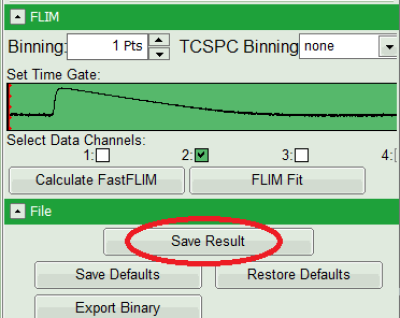
• Save the result by clicking on “Save Result”.

Response:
A result file (FLIM.pqres) is stored under the raw data file (CENP-labelled_cells_for_FRET.ptu).

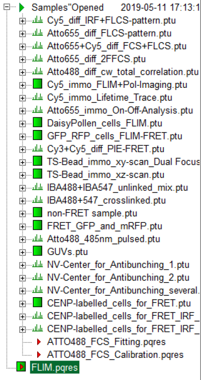
• Now the first part is finished and the FLIM window should be closed.

• Highlight the file CENP-labelled _cells_for_FRET.ptu again by a single mouse click.

• Select the “Analysis” tab and in there, open the drop down menu “Imaging”.

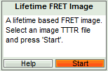
• Start the “Lifetime FRET Image” script by clicking on “Start”.

Response:
The “Lifetime FRET Image” script is applied to the file CENP-labelled _cells_for_FRET.ptu. Thereby, a new Window opens:

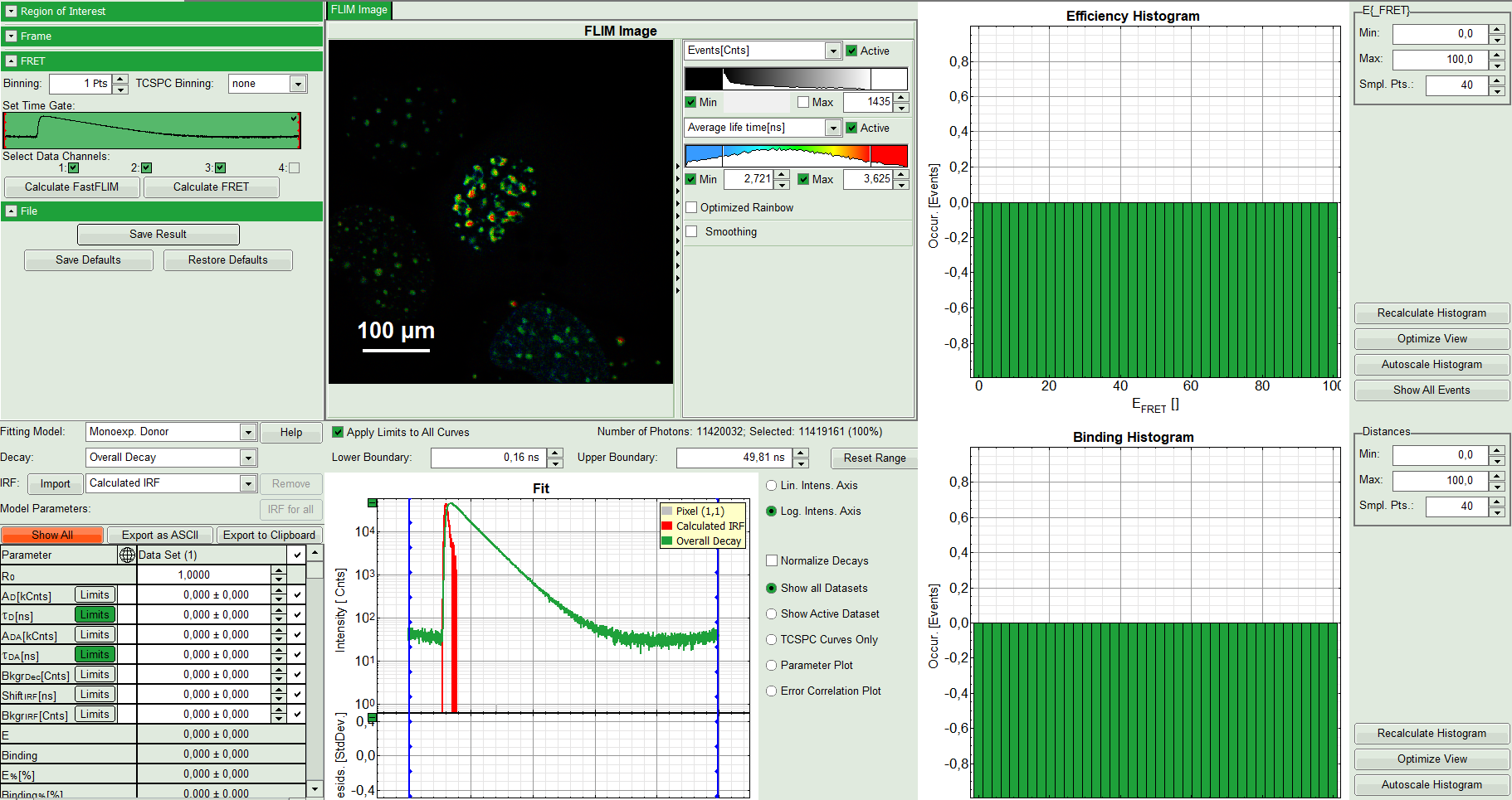
The window contains five different regions: Upper left: Imaging analysis options
Upper center: Fast FLIM image, displayed in false color scale. The brightness encodes the intensity while the color encodes the average “Fast FLIM” lifetime, i.e. the mean arrival times of the photons after the laser pulse. When not defined otherwise, intensity and color scale stretch from minimum to maximum. As the mean arrival time of the background photons in the areas where no fluorescence is detected, is randomly spread over the TCSPC window, the mean photon arrival time of the dark background is usually very long (up to 1/2 of the TCSPC window), which makes the color scale loaded by default sometimes unsuited for displaying the lifetime contrast in the actual sample. In this case, the scale has to be adapted.
Upper right: Fluorescence FRET Efficiency Histogram. As the FRET efficiency image has not been calculated yet, this plot is still empty. Later, the settings of the plot can be adapted using the controls on the right of the plot.
Lower left: Binding histogram. As the FRET efficiency image has not been calculated yet, this histogram is also still empty. As this diagram can only be calculated if the FRET donor dye has single exponential decay kinetics, changing the fitting model results in an exchange of this graph to a FRET distance histogram.
Lower center/left: TCSPC histogram of all photons in the image in green (= dataset 0) and the TCSPC histogram of a single pixel in grey (= dataset 1). In red an estimation of the instrument response function (=IRF) is shown. The IRF reconstruction is deducted from the rising edge of the images TCSPC histogram. On the left of this graph, the fitting model and parameter controls are displayed.

• Select only channel 2 as active channel.
• As the photon number/pixel is quite low in this image, select a Pixel Binning of 4 points.
• Press “Calculate FastFLIM” to update the image.

Response:
The pixel binning is applied to the image and the image is recalculated, using only photons from detector channel 2.

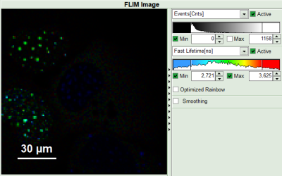
• Set the intensity scale from 0 counts – 200 counts and the lifetime scale from 0 to 5 ns.

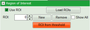
• On top left, under Region of Interest, check “Use ROI” box and click on “ROI from Threshold”.

Response:
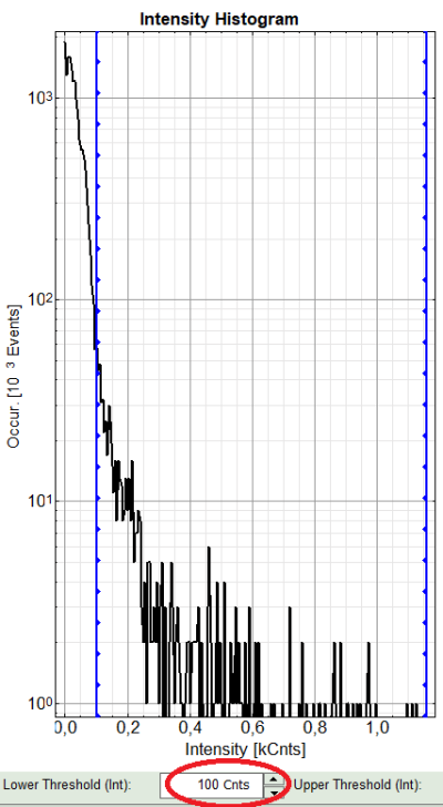
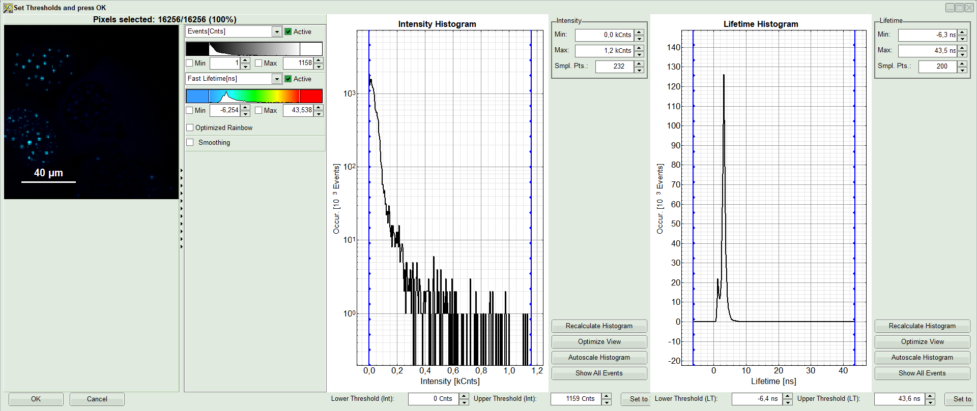
A large window with three sections will appear, where you can set a threshold for an image analysis visually.

Note:
Left to right: Preview FLIM Image, Intensity Histogram and Lifetime Histogram. For any ROI you can set each of these parameters individually. There are two ways to define the new threshold. You can use the edit-box at the lower side to type the threshold and press enter to check the result or use cursor keys or mouse wheel to increase/decrease the value. Another option is using the blue vertical bars on the sides of the intensity or lifetime histograms; click and drag the bars to set the threshold.

• In this example set the lower intensity threshold to 100 counts.

• Click “OK”

Response: In the image, only pixels with higher photon counts are highlighted. (eventually adapt the intensity maximum to see the highlighted pixels more clearly).

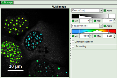
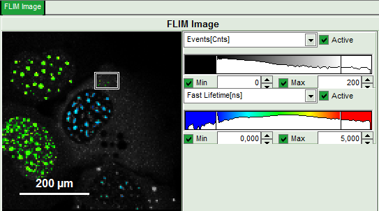
• For the analysis, only the spots within the nuclei of the cells are of importance. Therefore exclude the bright dots outside the nucleus of the cell on the lower right by placing the mouse cursor over the image, activate the context menu with a right mouse click, select “Rectangle ROI”, press continuously “CRTL” and draw rectangles around the spots outside the nucleus.
• Response: The marked regions are excluded from analysis.

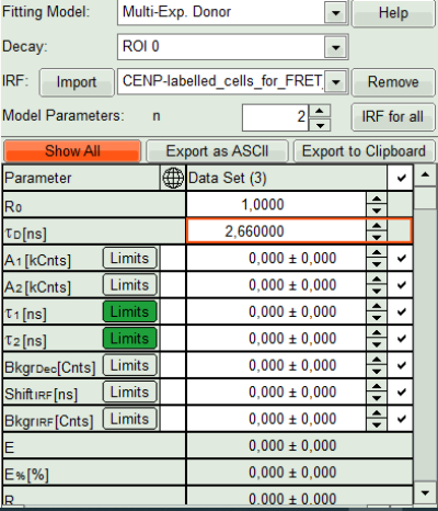
• In the lifetime fitting pannel, set the Fitting model to “Multi-Exp. Donor”.

• Click on IRF “Import”

• In the window appearing, select the file CENP-labelled cell_for_FRET_IRF_Det2.ptu as before in the FLIM script and click “OK”.

• Activate the imported IRF by choosing it in the IRF option (if not shown automatically).

Response:The imported IRF is highlighted in red.

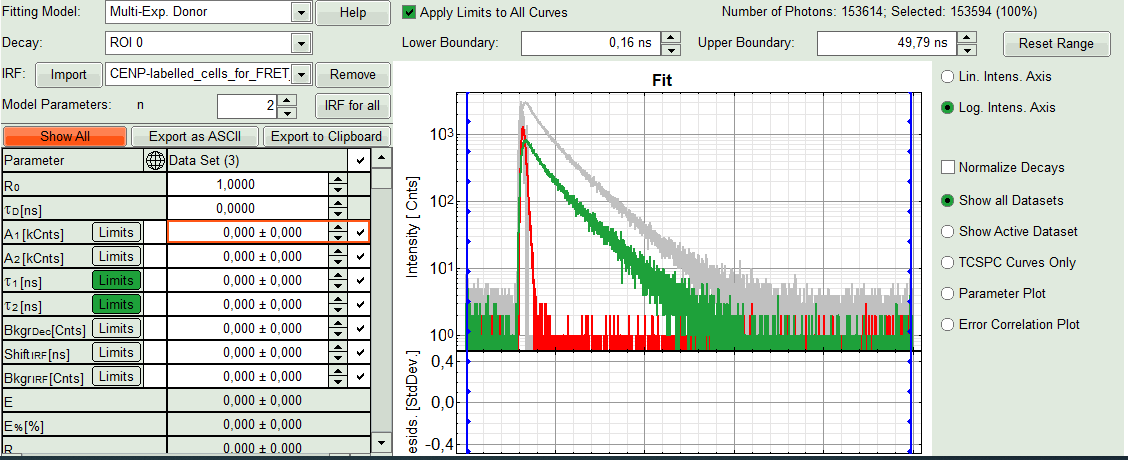
• As model parameters, select n=“2”.

Note:
If a mixture of complexes performing FRET and not performing FRET is present, the decay can of course be more complex, as the Cerulean alone already shows a bi-exponential decay behavior. However, the limited number of photons per pixel does not allow to use a more complex model.

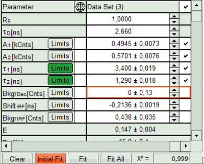
• In the parameter panel, enter “2.66” ns as τ_D.

Note:
Whether you need to type “2.66” or “2,66” depends on the country specific settings of Windows program. For this tutorial, a computer with German specific settings was used, therefore, the decimal digits are separated with “,” instead of “.”.

• Click “Initial Fit”.

Response:The fit is performed to the ROI decay.

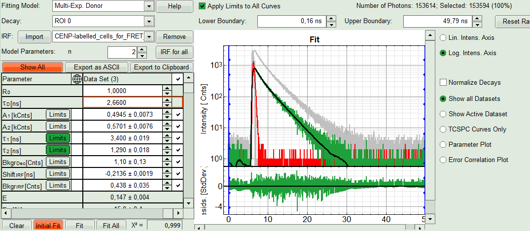
• In the Fitting panel, set the parameters Bkgr_Dec, Shift_IRF and Bkgr_IRF constant by removing the mark. Set the background of the decay to 0.

Note:
In order to reduce statistical fluctuations, as many parameters as possible need to be set constant. In a single pixel, the background counts of the pixel are negligible, therefore it is valid to set this to 0 in this case. Don't press “Initial Fit again”.

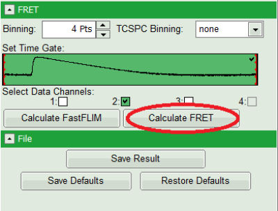
• Press “Calculate FRET” in the upper panel on the left.

Note:
Depending on the screen resolution, one may have to use the scroll-bar in order to access this button.

Response:

• A double exponential fit with the chosen start parameters is calculated for each selected pixel.
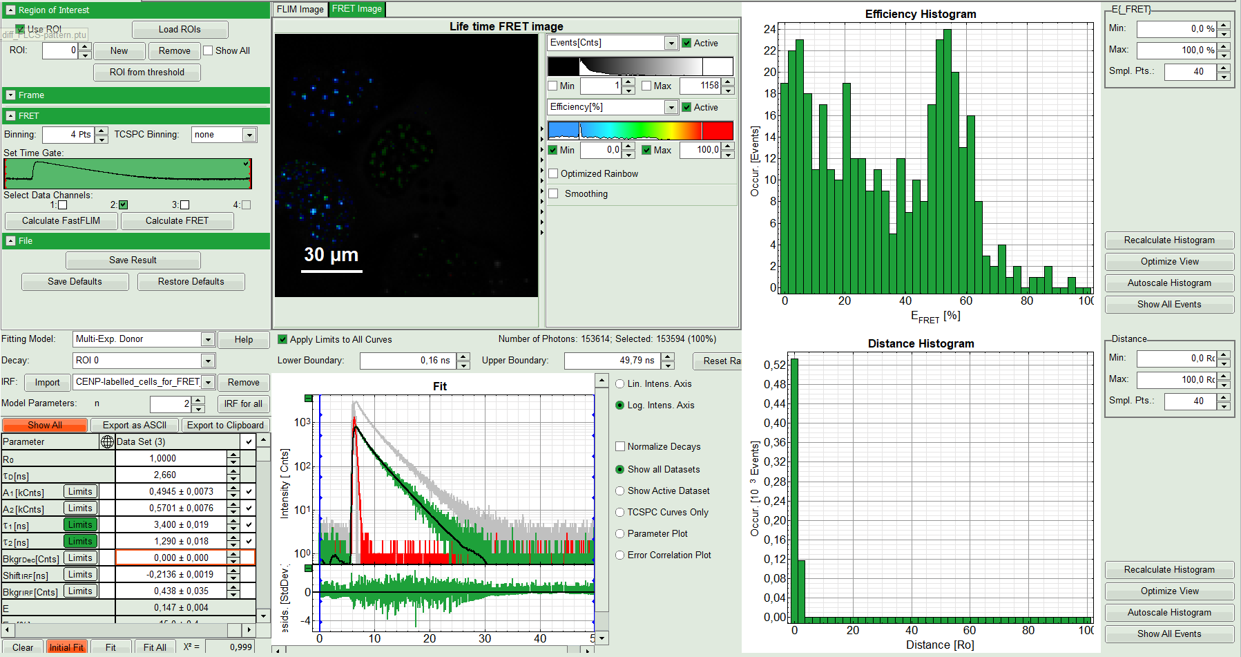
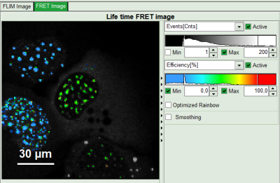
• From the results, a “FRET Image is calculated which is plotted in the FLIM image area. The FLIM image is hidden behind in another tab.
• On the right, the FRET efficiency histogram is plotted from the pixel values.
  • This graph shows 2 peaks, which is expected, as in the image one can see two cells with donor and acceptor construct and two cells without. For the cells with the FRET donor only, a FRET efficiency around 0 is expected and also shows up in the histogram.
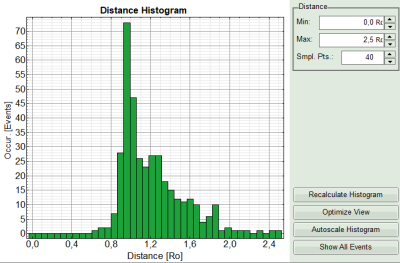
• On the lower right, the FRET distance histogram is plotted. As we didn't enter any value of the Förster distance R0, the distance is plotted in terms of “R0”.

• Adjust the intensity scale to 0 counts – 200 counts in order to better compare the lifetimes in the Donor-Only and the FRET-cells.

Note:
The FRET efficiencies calculated also show values below 0. Although physically impossible, mathematically this reflects the variation in the fit.

• Set the maximum for the distance in the distance histogram to 2,5 R0.

Note:
To transfer the distance into a nanometer scale, the real Förster distance must be known. The result is only meaningful, if the donor to acceptor ratio is 1:1 on the molecular level for each complex. This is not the case in our biological example with a more complex stoichiometry, therefore the graph is meaningless in this specific case.

Calculating the real Förster distance requires some effort and distinct knowledge about the sample. A few aids are available on the lab. These are not connected to PicoQuant and PicoQuant is not responsible neither for the content nor any possible errors; still these links may give an idea of what is required to calculate Förster distances.

• http://www.pymolwiki.org/index.php/Forster_distance_calculator

• http://www.osmanbilsel.net/software/forster-distance-calculator

• http://en.wikipedia.org/wiki/F%C3%B6rster_resonance_energy_transfer

• Press “Save Result” to save the current analysis.

Response:
A result file is saved and linked to the raw data file.

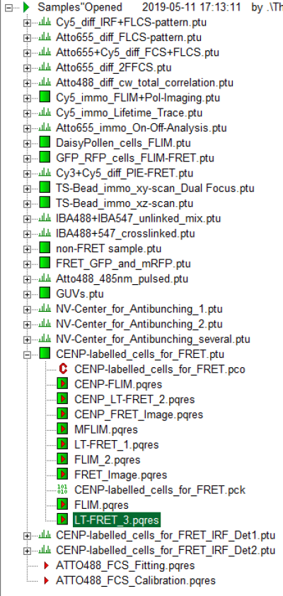
• The image analysis is now finished. There are several possibilities to continue:
  • To adapt the histogram plots, change the plot parameters on the right of the histogram to the desired values and click “Recalculate”. To save these plots, click “Save Results” again.
  • To export certain analyses, place the mouse cursor over the area of interest, activate the context menu with a right mouse click and choose the export function of interest to export the data.
  • To analyze many images with the same FRET pair, it is possible to save the starting values for the fits by clicking on “Save Defaults” and store the starting values as a User Profile by entering the main menu (“Settings\Save User Profile as”). The software will need to restart to adapt the changes.
• If you don't want to do anything more, just close the result window.