ROI Fitting Using the FLIM Analysis (updated for SymPhoTime v2.5)
Introduction
This tutorial shows step-by-step, how the FLIM script of SymPhoTime 64 can be used to fit several regions of interest (ROIs), and how to extract and interpret the results. In detail, the FLIM script is started using an image of mouse kidney tissue in the “Tutorials” workspace, https://figshare.com/s/4957fcfa684daef86c23, a suited fitting model is chosen and a pixel-by-pixel fit is performed.
Step-by-step Tutorial
Select a file and start the analysis
- Start SymPhoTime 64 software (this tutorial uses version 2.5, there might be differences when working with other versions).
- Open the “Tutorials” workspace via File → Open Workspace from the main menu.
Response:
The files of the sample workspace are displayed in the workspace panel on the left side of the main window.
- Highlight the file
Kidney_Cells_FLIM.ptuby a single mouse click. - Select the “Analysis” tab and in there, open the “Imaging” drop-down menu.
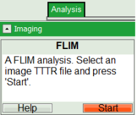
- Start the FLIM script by clicking on “Start”.
Response:
The FLIM analysis is applied to the file Kidney_Cells_FLIM.ptu. Thereby, a new Window opens:
Note:
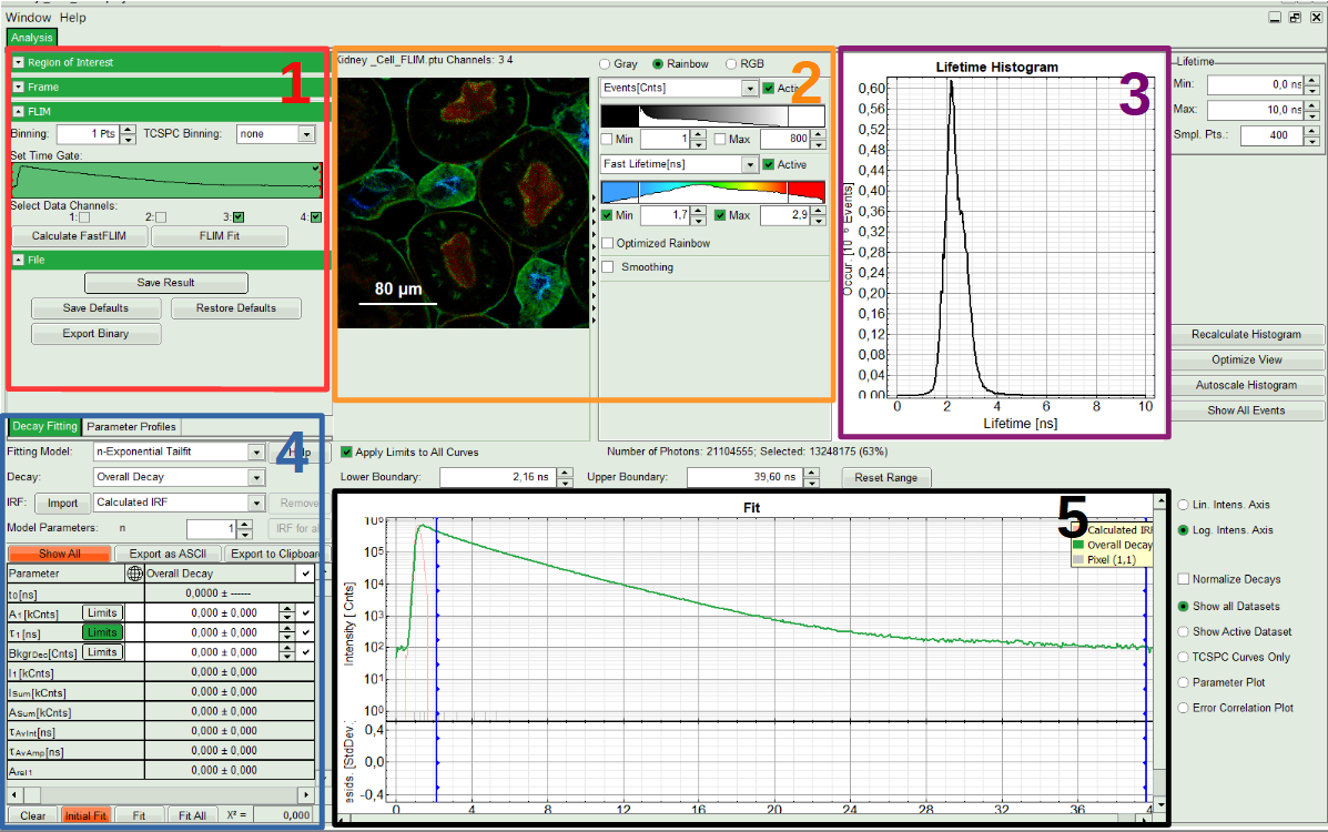
The window contains five different sections:
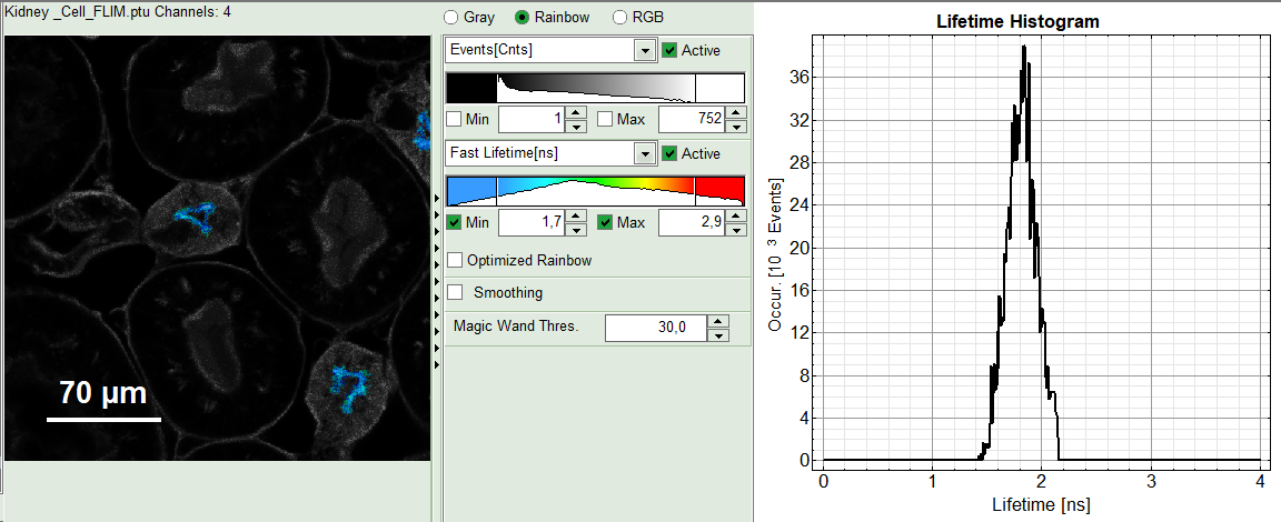
1: Setting panel
Imaging analysis options can be defined in this section.
2: Fast FLIM image
The FLIM preview image displayed in a false color scale. The brightness encodes the intensity, while the color encodes the average “Fast FLIM” lifetime, i.e. the mean arrival times of the photons after the laser pulse. When not defined otherwise, intensity and color scale stretch from minimum to maximum. As the mean arrival time of the background photons in the areas where no fluorescence is detected, is randomly spread over the TCSPC window, the mean photon arrival time of the dark background is usually very long (with an average up to 1/2 of the TCSPC window), which makes the color scale loaded by default sometimes unsuited for displaying the lifetime contrast in the actual sample. In this case, the scale can be adapted.
3: Fluorescence Lifetime Histogram
Here the frequency of photon counts corresponding to the individual mean lifetimes is plotted. The settings of the plot can be adapted using the controls on the right of the plot. The histogram is photon weighted.
4: Decay Fitting Parameters
Here the lifetime fitting model can be selected. Fitting is then applied to the lifetime graph(s) on the lower center (TCSPC histogram).
5: TCSPC Decay window
By default, this set shows the TCSPC histogram of all photons in the image in green (= dataset 0) and the TCSPC histogram of a single pixel in grey (= dataset 1). In red an estimation of the instrument response function (=IRF) is shown. The IRF reconstruction is deducted from the rising edge of the TCSPC histogram.
- To enhance the lifetime contrast, adapt the color scale by typing the limit values for the “Fast Lifetime [ns]” and “Events[cnts]”. Additionally set the “Lifetime Histogram” range on the right hand.
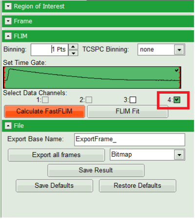
- Tick the checkbox of the detection “Data Channel” (i.e. detector), you want to use - in this case detector channel 4 - and press “Calculate FastFLIM”.
Response:
The FLIM Preview image will get updated. Optimize contrast by adapting “Min” and “Max” values.
Select a file and start the analysis
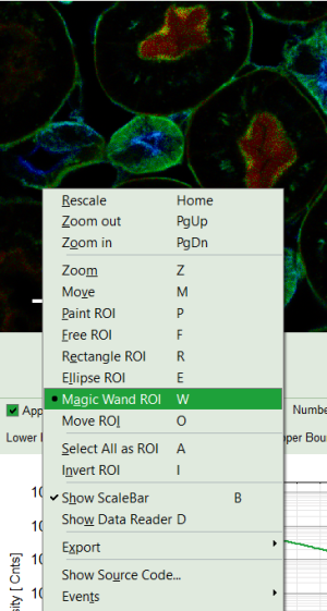
- In the FLIM preview image, ROIs can be selected using the context menu (Right Click).
Note:
- The following ROI-selection tools are available: Rectangle ROI, Ellipse ROI for simple drawing and Paint ROI for marking the pixels the mouse passed over. The faster the mouse pointer moves, the broader the marked lines will get. Free ROI draws a free shape. The pixels within the drawn shape will be selected. Finally Magic Wand marks area with similar fast lifetime.
- Using keyboard shortcuts
<CTRL>+<Z>you can undo a selection. Redo also with<CTRL>+<Shift>+<Z>is possible.
- You can add several areas to an existing ROI with the same or different selection tool by keeping the
<Shift>key pressed while drawing the additional regions.
- If you want to remove some of the pixels from the selected ROI, just keep the
<CTRL>key pressed when using a ROI selection tool to exclude the unwanted parts.
- Additionally you can zoom, move or Invert the ROI. Please see the shortcuts provided for each option in the context menu.
- If you want to start again from scratch select “Select all as ROI”.
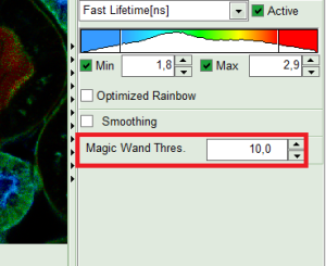
- In this step, as an example, we mark an ROI with similar lifetime range using the “Magic Wand” tool. The sensitivity of the tool to lifetime differences can be adjusted in a box below the intensity and color scale options.
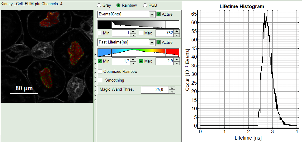
- Increase the threshold to 25.
Response:
The parts of the image with a similar fast lifetime range will be selected and the lifetime histogram will get updated accordingly. If you want to combine several spatially separated regions with a similar lifetime into one single ROI, as it's done here, you have to press “Shift” when selecting the spatial separated areas with the Magic wand tool.
Note:
Since this function is based on the displayed image, the sensitivity of the selection is dependent on the scaling of the color-encoded component. Changing the color scale (in general the lifetime) can change the sensitivity of this tool.
Response:
An extra gray decay corresponding to ROI 0 will appear under decay fit in “Decay Fitting” panel.
Note:
For fine adjustment, you can use any other ROI selection tools from context menu. In this case better to use <CTRL> or <Shift> buttons in order to remove pixel with a different or add pixels with similar fast lifetime. Ideally try to select an ROI with 10000 to 100000 counts in peak for getting the optimum statistics. ROIs with lower intensities can also be fitted, but in case of a more-exponential decay, some components might not be resolved.
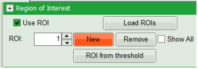
- In order to select an additional ROI, click “New” ROI.
Response:
The software assigns sequential numbers to selected ROIs.The whole preview image will appear again.
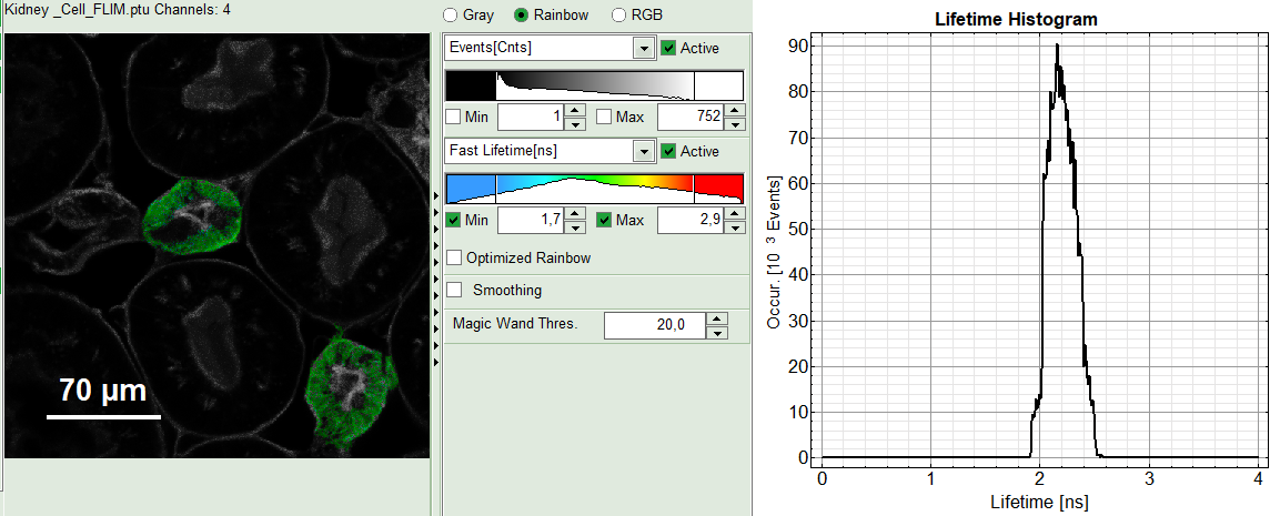
- For the next ROI, first we use the same tool, “Magic Wand” but adapt its threshold to 20.
- Repeat the last two steps in order to select the cell nuclei as the last ROI.
Response:
Now you can see fast FLIM (preview) images of “ROI 0”, “ROI 1” and “ROI 2” when selecting them in the ROI-list In the Region of Interest-Menu, as well as their corresponding decays in TSCPC window in grey when selecting the different decays in the list.
Perform an Initial Lifetime Fit on the Selected Regions (ROIs)
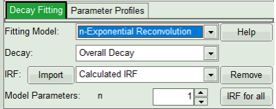
- In the forth box, “Decay Fitting”, from the Fitting Model drop-down list select “n-Exponential Reconvolution Fit”.
Response:
In the TCSPC window, the IRF is displayed in bright red, the data fitting limits are moved to the border of the TCSPC window.
The new fitting parameters “Shift IRF” and “Bkgr IRF” (=background IRF) appear in the fitting parameter table.
Note:
The software offers the possibility to fit the data using an n-exponential tailfit, n-exponential reconvolution or rapid reconvolution fit. A tailfit can be used when the fitted lifetimes are significantly longer than the instrument response function. A reconvolution fit is usually preferable, because the complete decay is fitted, while for a tailfit, the start of the fitting range is usually a bit arbitrary. A rapid reconvolution fit is suited, if the image was measured with a very high countrate and a system with a dead time significantly above the pile-up-limit or when the image has been acquired with a repetition rate, which is normally too high for the lifetime of the dye, so that the decay is not at the background level at the end of the decay window. The rapidFLIM-fitting is explained in another tutorial.
For explanation about the fitting model and the used equations, click on the “Help” button next to the selected model. This opens a help window containing the fitting equation and the explanation of the different parameters.
- From “Decay” drop-down list select
ROI 0and click “Initial Fit” (marked in orange).
Response:
A single exponential reconvolution fit is performed. In the TCSPC window, the fit is displayed as a black line. Below, the residuals (= difference between raw data and fit values) are displayed.
- Fit values appear in the fitting table. Check the fitting curve, residuals and χ².
Note:
Usually, a decent fit is characterized by the following criteria:
The fitted curve overlays well with the decay curve. In the residual window, the values spread randomly around 0.
The χ²-value approaches 1.
The calculated fitting values are reasonable.
The fitting model with least parameters is preferred.
- In this example it is obvious that the applied single exponential reconvolution fit is not suited to fit the decay curve. Increase the “Model Parameters” to n = 2. Again, click on “Initial fit”.
Response:
The fit quality increases. But if it still doesn't look sufficient. One sees a trend in residuals and not a random distribution around 0. Increase number of “Model Parameters” to three.
- Here the fitting model shows a satisfying result. A 3-exponential fitting model should be used for ROI 0.
- Try the last two steps with “ROI 1”.
- Find the best fit for “ROI 2” in a same manner. It is better always to start from monoexponential and try to find the fitting model with a lower number of components.
- Three components exponential decay seems to be suitable for all three ROIs. If all ROIs can be fitted with the same model, you can also click on “Fit All” to get all curves fitted with the same model.
- Clicking on “Fit All” will fit all active data sets with the same model, using the start parameters of the active data set. If you do not want to fit the complete decay (dataset 1) and the decay of a single pixel (Dataset 2), press “Show All” button:
- Uncheck the first two datasets on top of the parameter table and press “Fit All” again.
Compare the lifetimes and save results
- In order to compare the lifetime of these three compartments, apart from fitting parameter table shown above, you can plot them by selecting the “Parameter Plot” on the right side of TCSPC window.
Note:
The X-Axes is showing the “Dataset Number” corresponding to the dataset listed in Decay drop-down menu (in Dcay Fitting Panel). This means by default “Overall Decay” and “Pixel (0,0)”, and then selected ROIs.
For the Y-Axes one can select one or multiple fit parameters.
- Tick the “tau_Av_Int” checkbox for Y-Axes and zoom in to be able to see the lifetime differences better.
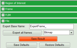
- At the end, click on “Save Result” button in parameter panel.
Response:
A result file “FLIM.pqres” is stored under the raw data file Kidney_Cell_FLIM.ptu.
- Later, clicking on the result file reopens the file in the same way as it was stored.
