Reconvolution fit
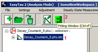
Select an .etc container that contains at least one IRF histogram and at least one decay curve. Open the Fitting Window by pressing ![]() .
.
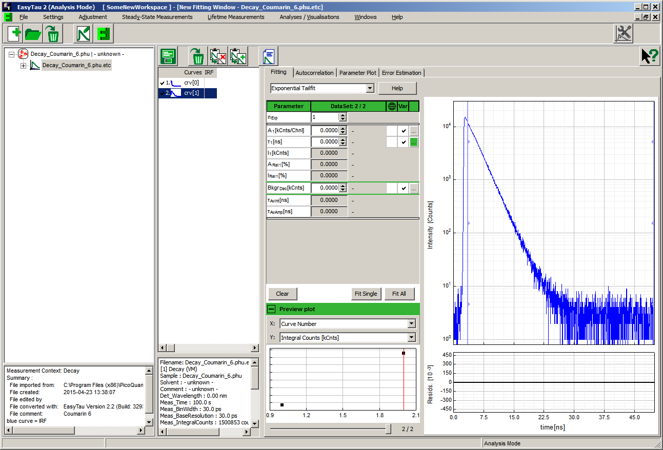
The last curve in the container, crv[1], a decay curve in this case, is displayed. The default fitting option is “Exponential Tailfit”. In order to perform a reconvolution fit, we need to select and then assign a curve as an IRF and then change the fitting modality.
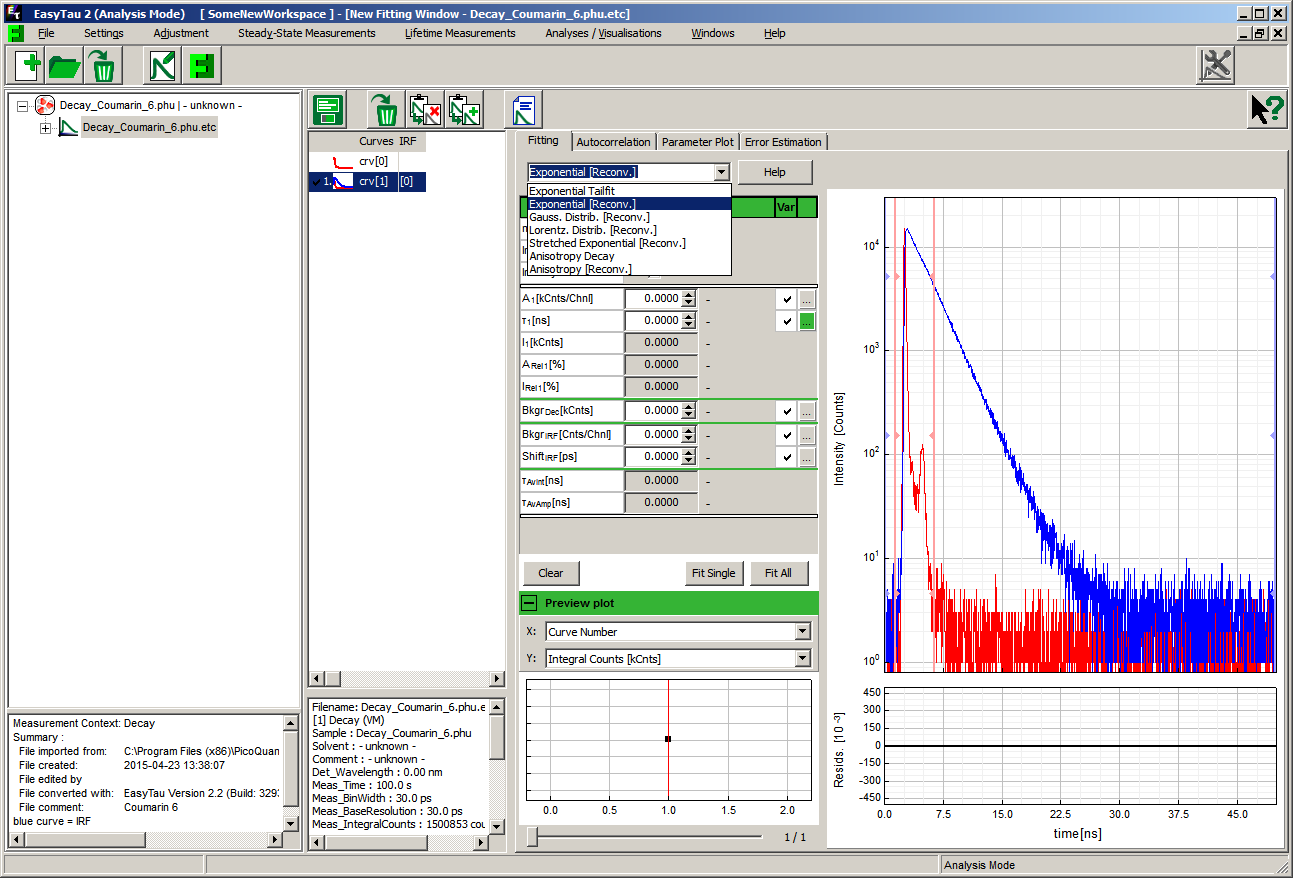
Clicking on (selecting) crv[0], the first histogram, the IRF in this particular case, updates the plot. Now, a right-click on crv[0] opens a context sensitive dialog, where the “Curve type” can be changed from “Decay” to “IRF”.
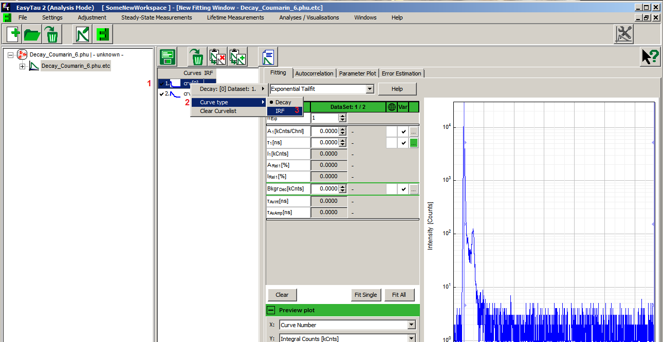
The plot is updated again. After these actions the fitting model can be changed to “Exponential [Reconv.]”
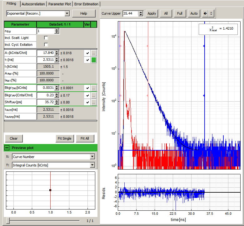
If necessary, change the time axis limits by dragging the appropriate vertical sliders in the plot. There are dedicated sliders for both IRF and decay curve time ranges. Pressing the “Fit Single” button performs a fully automated fit of a single exponential decay model:
This simple model is entirely appropriate for this particular decay curve. However, the complexity of the model can be increased by adding more exponential terms (nExp) or activating the correction for scattered light or cyclic re-excitation. The mathematical formulas and definition of terms is available by pressing the “Help” button inside the fitting dialog. It is possible to fix any parameter of the fitted model by removing the corresponding tick in the “Var” column.
An introduction to the basic principles can be found in this manual of the predecessor of EasyTau2, the now discontinued FluoFit.
