Pattern Matching
Summary
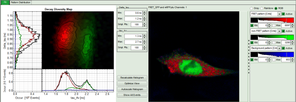
Pattern Matching Analysis by decomposing a recorded image into different user-defined patterns. Display of the calculated data using an RGB false color model. The calculated amplitudes of the first three defined patterns are depicted in three different colors for each pixel.
Open an Image
The following steps describe how to perform a Pattern Matching Analysis on raw data. This allows for separating different dyes or regions of different lifetime/decay-behavior in a sample.
- Copy the sample workspace from the DVD to a local disc drive and open it.
Response: The sample workspace contains several examples of measurements and analyzes. The files of the sample workspace are displayed in the workspace panel on the left side of the main window.
- Click on the file
FRET_GFP and mRFP.ptu.
Response:
- The file is highlighted in the workspace tree view.
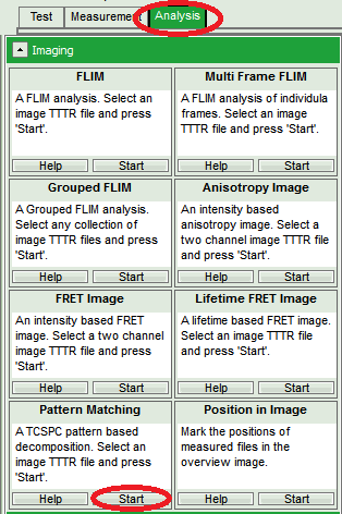
- Open the Imaging drop down window of the Analysis working mode and press the Start button of the Pattern Matching box.
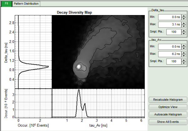
Response: The software calculates a Decay Diversity Map, a simple intensity image and an overall decay from the raw data file.
Select Patterns
Note: Once an image is generated, the next step is to select the patterns which are to be used for decomposing the image.
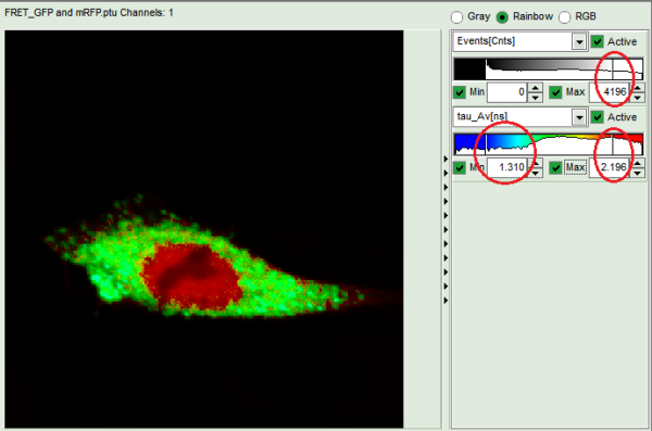
- Variate the settings of the Rainbow-image via the sliders for intensity and lifetime to enhance the contrast between the different regions.
Response: The image now clearly shows two populations of different lifetimes. This means, that probably two patterns are sufficient to fit the image.
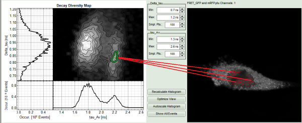
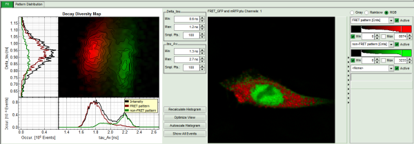
Note: Have a look at the Decay Diversity Map. This new feature tells you more about the different populations in the picture. The Decay Diversity Map is a 2D histogram. The x-axis shows a histogram of the average lifetimes of the pixels in the image. The y-axis shows a histogram of the Delta-Tau values of each pixel in the image.
This quantity relates to the deviation of the fluorescence decay from a mono-exponential decay. While a small value depicts a mono-exponential decay, a bigger Delta-Tau value indicates a multi-exponential one.
Note: In the example, two peaks in the average lifetime (x-axis) can already be seen.
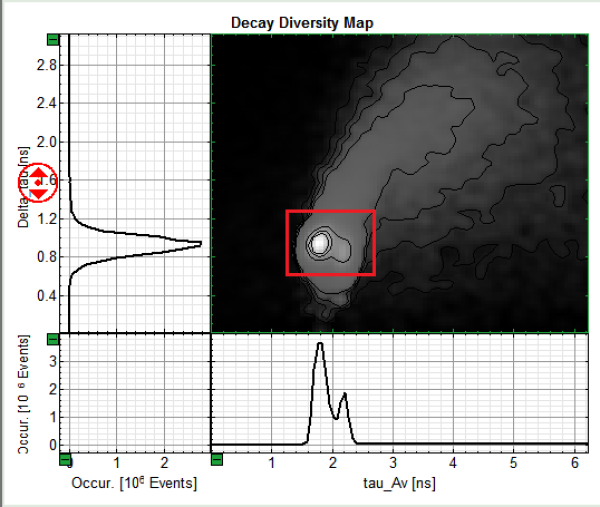
- Zoom into the Decay Diversity Map to see the two different populations and their different lifetime-properties.
Response: The zoomed region is now displayed in the same resolution as before.
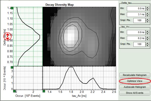
- Click the Optimize View button to enhance the resolution.
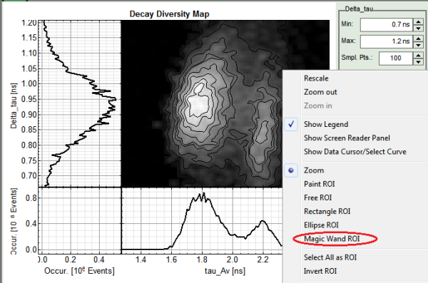
Response: More detailed contour lines are displayed. In our example the two populations and their different properties are depicted. The first population has a shorter lifetime and a slightly bigger Delta-Tau value compared to the second population. This indicates the first one to be the FRET population, as the lifetime is shorter and the decay “less” mono-exponential. The bigger deviation from mono-exponentiality results from the fact, that the molecules in question are composed of a mixture of one population performing FRET and an additional population of Donor-only or non-FRET molecules. The second therefore is the non-FRET population without any FRET performing molecules.
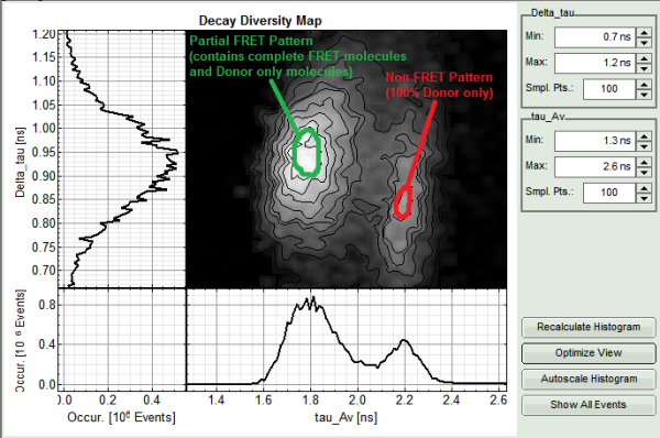
- In the right-click menu select the magic wand ROI (region-of-interest).
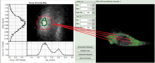
- Select the innermost contour line by clicking on it.
Response:
- The selected ROI is highlighted in the Decay Diversity Map. Also the location of the selected pixels in the intensity image is depicted.
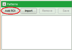
- Click Add ROI in the Patterns box.
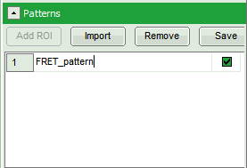
Response: The selected ROI appears as pattern in the box and its overall decay is displayed in the Patterns plot.
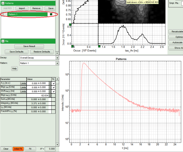
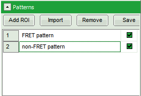
- Rename the pattern by clicking on it. Change the name to “FRET pattern”.
- Now repeat steps 5-8 to add the second population as “non-FRET pattern” to the list of patterns.
Response: Both decay-patterns appear in the Pattern box and in the Patterns diagram.
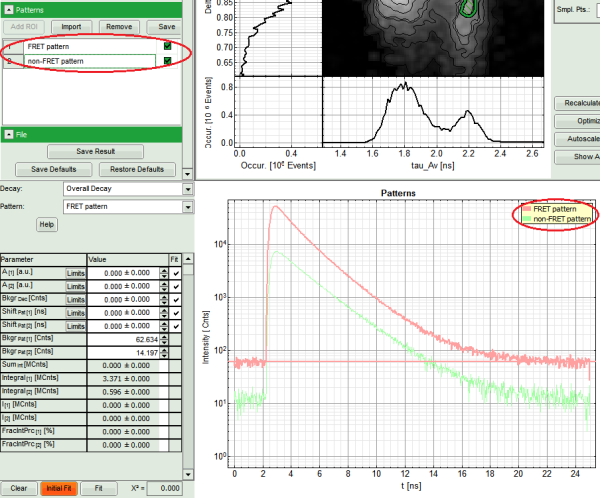
Note: Another option to acquire the patterns would be to select the different populations in the intensity image also using the magic wand ROI. Several non-connected regions can be selected by pressing the Shift-key while clicking. The procedure resembles the one described above.
Patterns can also be imported from other measurements. For more details, see Additional Information at the end of this step-by-step manual.
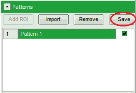
Patterns can be saved by simply clicking the save button in the Pattern box. This allows for analyzing them with the TCSPC Fitting feature and calculating the values of the average FRET efficiency and binding (not shown).
Perform a Pattern Fit
Note: The desired patterns are already selected (in the example the FRET and the non-FRET pattern) and can now be used for fitting.
It is recommended to perform an initial fit before starting the Pattern Fit. This is because some parameters of the initial fit will be used in the Pattern Fit as start parameters and also because an initial fit is a good indicator, whether the defined patterns suffice to describe the image.
The initial fit  feature decomposes the overall decay (average over all pixels) into the user-defined patterns. This is done in terms of a linear combination. In general, for i Patterns it finds the corresponding amplitude αi:
Decayoverall = Σi αi ( Patterni - Bkgri )
In addition, a shift parameter can shift the decay in time.
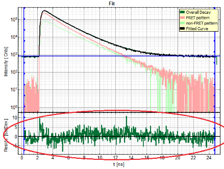
If the residuals of the initial fit show no trend or outliers, it is safe to assume that the selected patterns suffice to describe the image and a Pattern Fit can be started.
Note: The Pattern Fit  algorithm is similar to the initial fitting one, but instead of decomposing the overall decay, it performs the decomposition on each pixel. The linear decompositions of the particular pixels give different αi's for every pixel.
After the fitting process a false color RGB image is displayed which shows the amplitudes αi of the first three patterns in three different colors for each pixel.
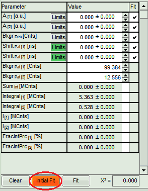
- Since the patterns are taken from the same measurement as the overall decay, it is justified to first set the Limits of the Shift values to 0, as there shouldn't be any shifts. (Unselecting the Fit-boxes doesn't prevent the plot-procedure from fitting the Shift values by pressing “Inital Fit”).
- Clicking Initial Fit will perform a fit for the overall decay (all photons of the image) by mixing the different patterns. As standard a Monte-Carlo search algorithm will be followed by a MLE optimization procedure.
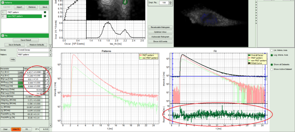
Response: Both decay-patterns, the overall decay and the resulting curve are displayed in the Fit diagram. The residual plot on the bottom should show no trends or big deviations in comparison to its noise level. This result shows that the image can be readily described by two different decay patterns belonging to two different species, the FRET and non-FRET population. The result would be even better by adding a background pattern (see Additional Information at the end of this step-by-step manual). From this result we can learn that the FRET pattern is composed of FRET molecules with only one specific FRET efficiency. Molecules with a different efficiency would result in deviations of the residual-curve and the need of a third pattern.
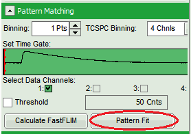
- Start fitting the image by pressing Pattern Fit in the Pattern Matching box. This process may take several minutes.
Response: The intensity image will be replaced by a pattern-fitted image. In this image the decay of each pixel is fitted by mixing the patterns. The pixel color is dominated by the most prominent pattern in the pixel-decay. In the Decay Diversity Map the location for each pattern is depicted in the same color as in the image.
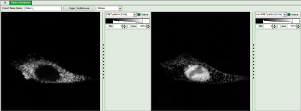
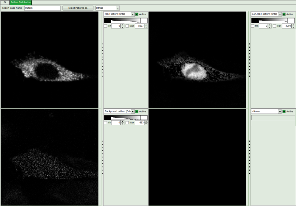
- Pressing Pattern Distribution shows black and white intensity images for the patterns, visualizing the most prominent regions of each pattern.
Additional Information
Note: There is a lot of possibilities to tailor the Pattern Matching Analysis to your needs and the given sample. Here are some examples using the same demonstration sample as above.
If decay measurements of the different components are available, one can also import patterns from different measurements.
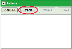
- To import a non-FRET pattern in our example: Click Import in the Patterns box.
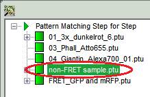
- In the pop-up window, select the reference-measurement (in the example select
non-FRET sample.ptu) and confirm by clicking OK.
Note: This will import the overall decay of the reference measurement. Make sure the measurement contains only the desired component. To make a better selection of the pattern to be imported, open the external measurement (in the example “non-FRET sample.ptu”) in another Pattern Matching Analysis and follow the step-by-step instructions to extract the desired non-FRET pattern.
- After selecting this pattern, click Save in the Patterns box.
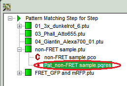
- Close the Analysis and import the saved pattern in the main analysis as described above, but instead of “non-FRET sample.ptu” select the created pattern (
Pat_non-FRET sample.pres).
Response: The imported pattern appears in the Pattern box and its overall decay is displayed in the Patterns plot.
Note: The fit of the overall decay can be improved by using a background pattern besides the patterns for the different regions.
- Extract the two patterns as described above and add them to the list of patterns.
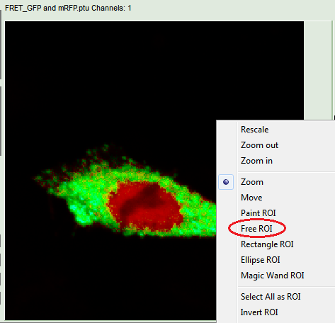
- Select the Free ROI tool in the right-click menu in the intensity image.
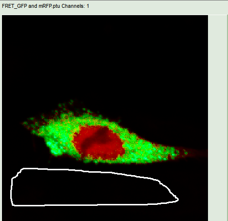
- Mark a region in the black part of the image to extract a background pattern.
Response:
- The selected ROI is highlighted in the intensity image (although hardly visible at standard settings). Also the location of the selected pixels in the Decay Diversity Map is depicted.
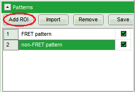
- Click Add ROI in the Patterns box.
Response:
- The selected ROI appears as pattern in the box and its overall decay is displayed in the Patterns plot.
- Rename the new pattern by clicking on it. Change the name to “Background pattern”.
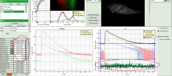
- Limit the Shift values to 0 and perform an initial fit as described in the step-by-step instructions, section Perform a Pattern Fit.
Response:
- All pattern decays, the overall decay and the resulting fit are displayed in the Fit window. The residuals are better than before, as they show no trends or waves at all, but only noise.
- Start fitting the image by pressing Pattern Fit in the Pattern Matching box. This process may take several minutes.
Response: The intensity image will be replaced by a pattern-fitted image. In this image the decay of each pixel is fitted by mixing the patterns. The pixel color is dominated by the most prominent pattern in the pixel-decay. In the Decay Diversity Map the location for each pattern is depicted in the same color as in the image.
- Pressing Pattern Distribution shows black and white intensity images of each pattern showing the most prominent regions of each pattern. The Background is now displayed in the third image.

