Table of Contents
Lifetime-Fitting Using the Rapid Reconvolution Model
Introduction
This tutorial shows step-by-step, how to use the Multi-Exponential Reconvolution fitting model with correction for rapidFLIM. This new approach allows better fitting for data acquired with rapidFLIM capable hardware with count-rates way beyond classical pile up limit.
For the principle of rapidFLIM - recording, check the application note available here: Application Note: rapidFLIM.
Here in detail the FLIM analysis of SymPhoTime 64 is used to perform a lifetime fit and how to extract and read the results. A mixture of Dragon Green and Nile Red fluorescent microspheres were imaged with more than three frames per second. Tutorials workspace can be downloaded from https://figshare.com/s/4957fcfa684daef86c23.
Step-by-Step Tutorial
Select a file and start the analysis
- Start SymPhoTime 64 software (This tutorial uses version 2.5).
- Open the “Tutorials” workspace via File → Open Workspace from the main menu.
Response:
The files of this workspace are displayed in the workspace panel on the left side of the main window.
- Highlight the file
MicroBeads.ptuby a single mouse click.
- Select the “Analysis” tab and in there, open the “Imaging” drop-down menu.
Note:
The drop-down menu can be opened and closed by clicking on the grey button on the left side of the header of the drop down menu:
- Start the FLIM analysis by clicking on “Start”.
Response:
The FLIM analysis is applied to the data file. Thereby, a new Window opens:
Note:
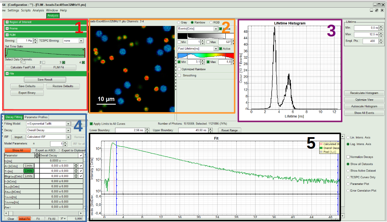
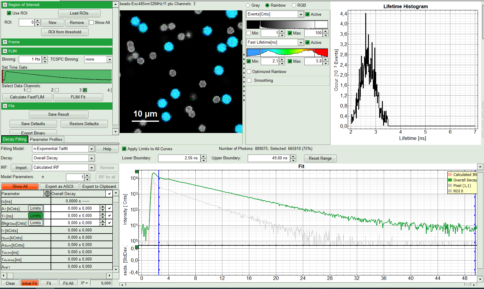
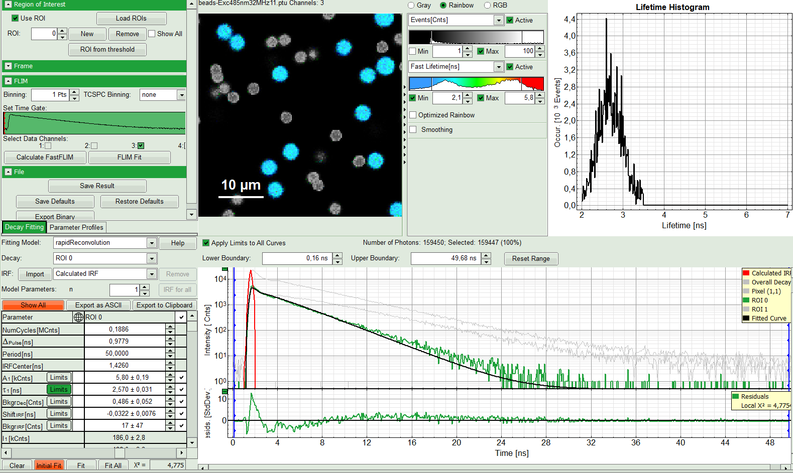
The window contains five different sections:
1: Setting panel
Imaging analysis options can be defined in this section.
2: Fast FLIM image
The FLIM preview image displayed in a false color scale. The brightness encodes the intensity, while the color encodes the average “Fast FLIM” lifetime, i.e. the mean arrival times of the photons after the laser pulse. When not defined otherwise, intensity and color scale stretch from minimum to maximum. As the mean arrival time of the background photons in the areas where no fluorescence is detected, is randomly spread over the TCSPC window, the mean photon arrival time of the dark background is usually very long (with an average up to 1/2 of the TCSPC window), which makes the color scale loaded by default sometimes unsuited for displaying the lifetime contrast in the actual sample. In this case, the scale can be adapted.
3: Fluorescence Lifetime Histogram
Here the frequency of photon counts corresponding to the individual mean lifetimes is plotted. The settings of the plot can be adapted using the controls on the right of the plot. The histogram is photon weighted.
4: Decay Fitting Parameters
Here the lifetime fitting model can be selected. Fitting is then applied to the lifetime graph(s) on the lower center (TCSPC histogram).
5: TCSPC Decay window
By default, this set shows the TCSPC histogram of all photons in the image in green (= dataset 0) and the TCSPC histogram of a single pixel in grey (= dataset 1). In red an estimation of the instrument response function (=IRF) is shown. The IRF reconstruction is deducted from the rising edge of the TCSPC histogram.
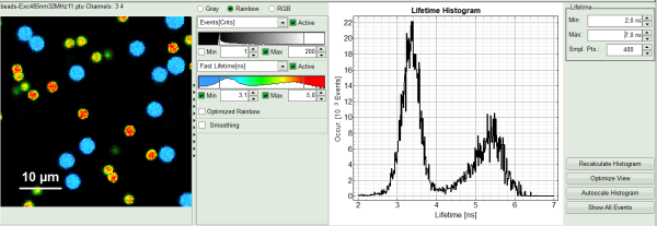
- To enhance the lifetime contrast, adapt the color scale by typing the limit values for the Fast Lifetime color scale. Additionally set the lifetime range for histogram on the right hand.
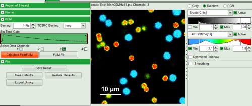
- Set Proper Detection Channel, in this case 3, and press “Calculate FastFLIM”.
Response:
FLIM Preview image will get updated. You may need to adapt the contrast again. Optimize contrast by adapting “Min” and “Max” values.
Select ROIs
- On top left, under Region of Interest, check “Use ROI” box and click on “ROI from Threshold”.
Response:
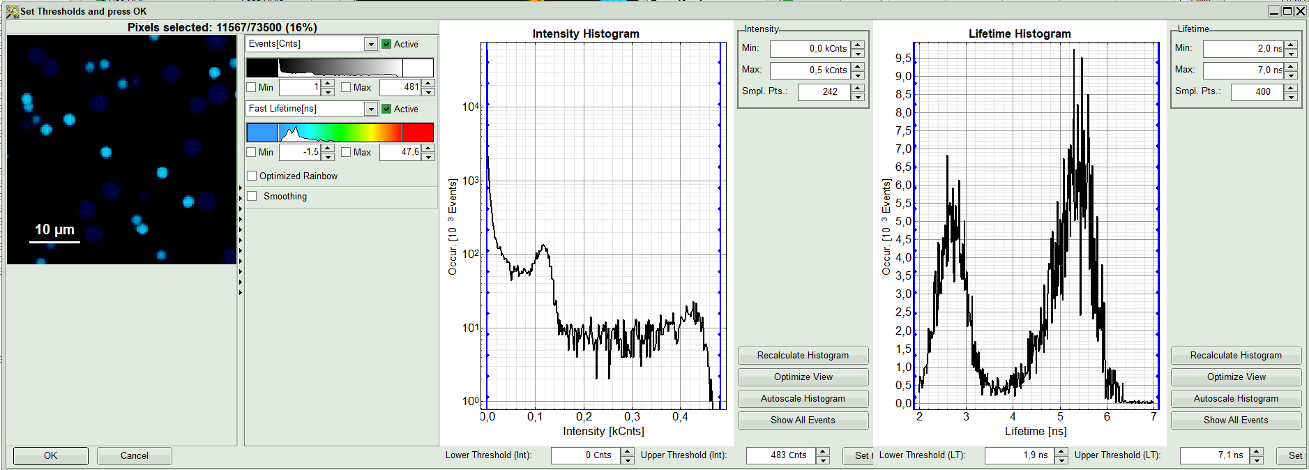
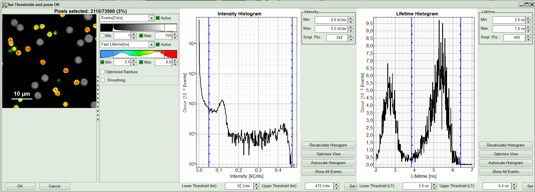
A large window with three sections will appear, where you can set a threshold for an image analysis visually.
Note:
Left to right: Preview FLIM Image, Intensity Histogram and Lifetime Histogram. For any ROI you can set each of these parameters individually.
There are two ways to define the new threshold. You can use the edit-box at the lower side to type the threshold and press enter to check the result or use cursor keys or mouse wheel to increase/decrease the value. Another option is using the blue vertical bars on the sides of the intensity or lifetime histograms; click and drag the bars to set the threshold.
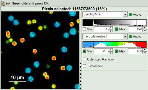
- First adapt the contrast by setting the Number of Events [Cnts] in brightest pixel and Fast Lifetime color code. This will help you to select your ROI or threshold easier.
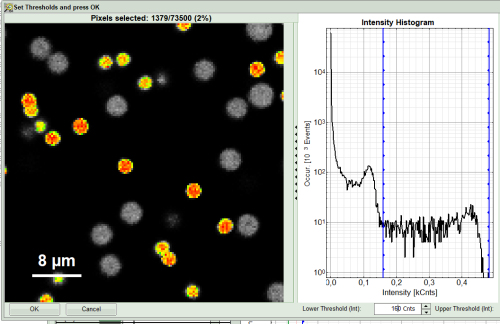
- As a next step try to distinguish compartments of your specimen in FLIM image by setting the intensity or lifetime thresholds. For instance select the area with higher intensity by dragging the indicator bars.
- Or try different lifetime range:
- Click OK to select it as the first Region of Interest.
Response:
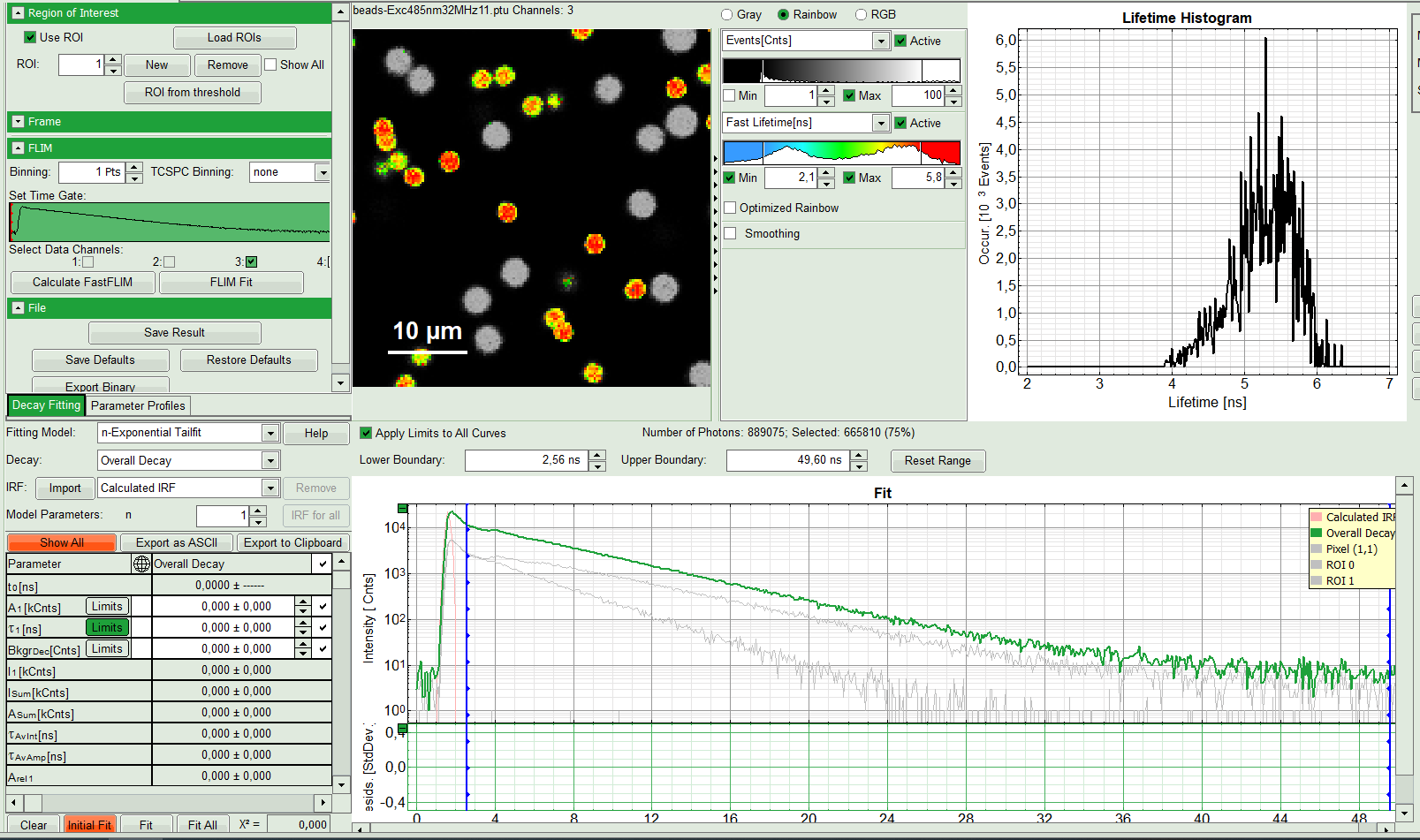
You will see ROI 0 on the top left window and an extra gray decay on bottom right under Fit. Lifetime histogram and the preview FLIM image remains as it has been selected in last step.
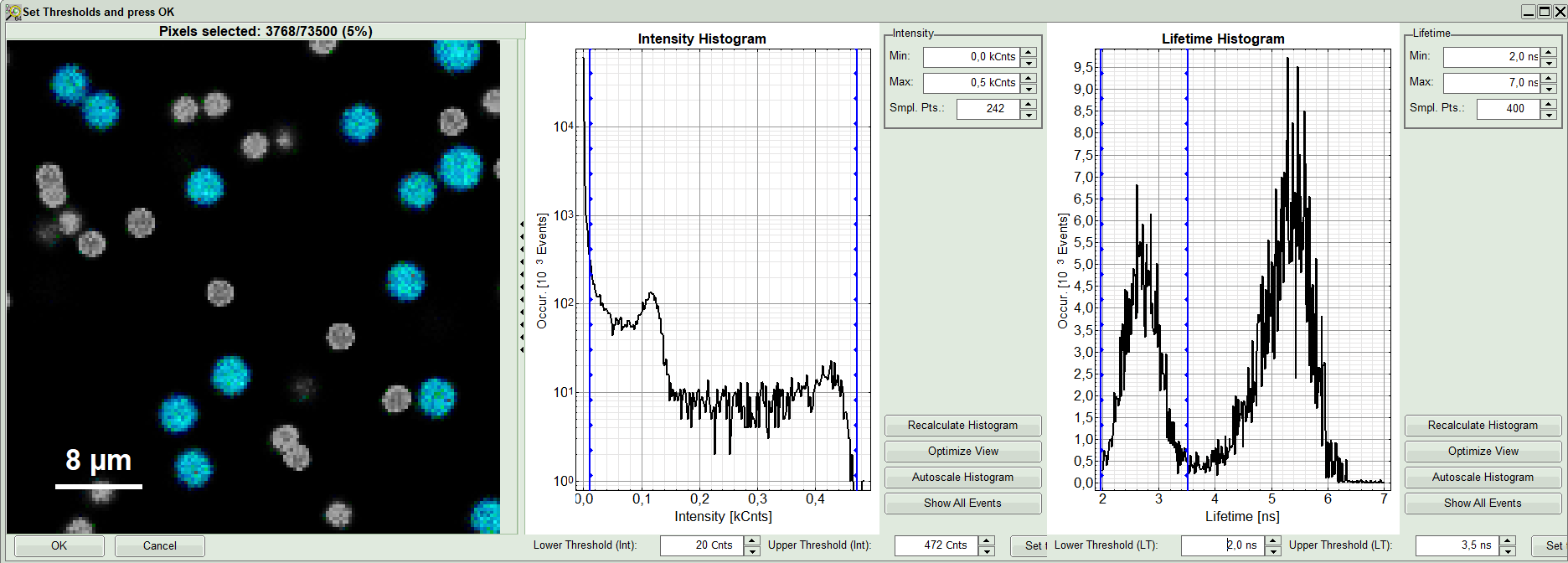
- In order to select an additional ROI, click on “New” ROI. The software gives sequential order numbers to your ROIs, so here ROI 1. The whole preview image will appear again. Define intensity and lifetime thresholds to select your new ROI.
- As an example here an area with longer lifetime is selected.
- When you are satisfied with your selection, press “OK”.
Response:
Corresponding decays with gray color will appear under Overall Decay curve.
Note:
Intentionally for this tutorial, the image was recorded at very high count rates using fast TCSPC electronics. We must consider distortion of the decay due to limited pulse pair resolution of the photon detector; Even the best detector cannot deliver infinitely narrow output pulses. At increasing count rates there is an increasing likelihood that two or more such detector pulses will overlap and merge into one. The counting and timing system can then no longer resolve the individual photon events and counts them as only one. Since the highest likelihood of such overlapping pulses exists at the peak of the decay curve, immediately upon excitation, one sees statistically more frequent loss of early photon counts rather than the late ones. As a consequence, the measured decay curve is increasingly rounded at its peak followed with a few ``bumps``. In order to exclude this detector artifacts for data analysis, rapid Reconvolution correction model estimates the loss probability in each channel and incorporates it into the fitting model.
Select the fitting model and determine start parameters
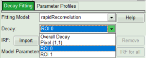
- On bottom left, in the “Decay Fitting” window, select the “rapidReconvolution” model. In the decay drop down list you will see the selected ROIs as well.
- Start with ROI 0 and only one component (monoexponential) fit. Press “Initial Fit” (marked in orange).
Response:
A single exponential fit is performed. In the TCSPC window, the fit is displayed as a black line. Below, the residuals (= difference between raw data and fit values) are displayed. Fit values appear in the fitting table.
Check the fitting curve, residuals and X².
For explanation about the fitting model and the used equations, click on the “Help” button next to the selected model. This opens a help window containing the fitting equation and the explanation of the different parameters.
- If the fitted curve is not overlaid not so well with the decay curve, like in this case, increase the “Model Parameters” to n = 2. Again, click on “Initial fit”.
Response:
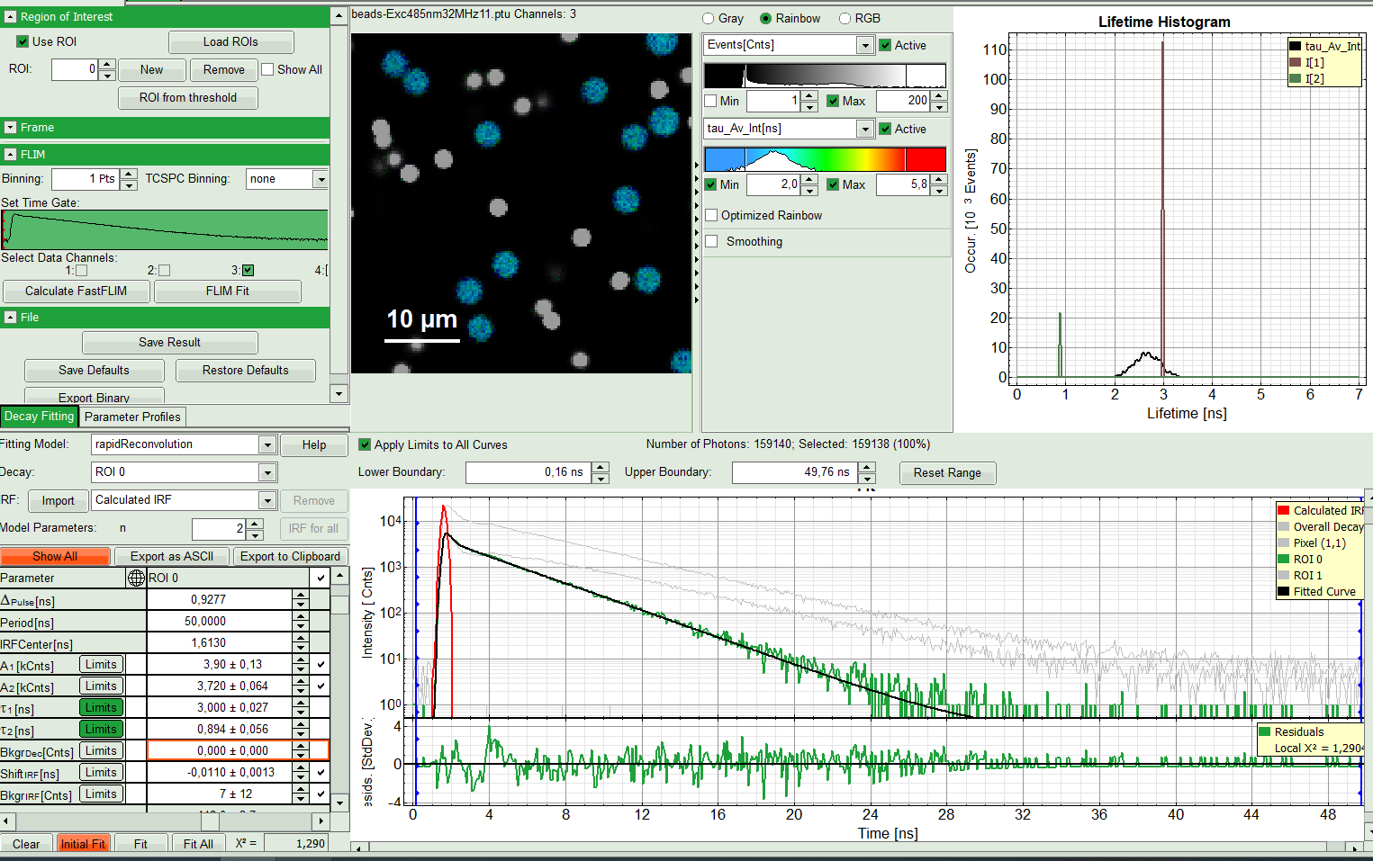
The fit quality increases. In the residual window, the values spread randomly around 0. The calculated fitting values are reasonable. The χ²-value got improved.
Note:
Usually, a good fit will be evaluated by residuals evenly distributed around zero and χ² approaches one.
However in such cases with systematic errors, one should not insist on getting ideal χ²- or residual values. The systematic distortions will introduce a slight systematic error in the fitted parameters, which will be negligible for exponentials that have a lifetime longer than the time constant of the systematic errors.
- Try last two steps with the ROI 1.
- Again a monoexponential fitting function is not sufficient. Therefore, we carry on with two components.
Response:
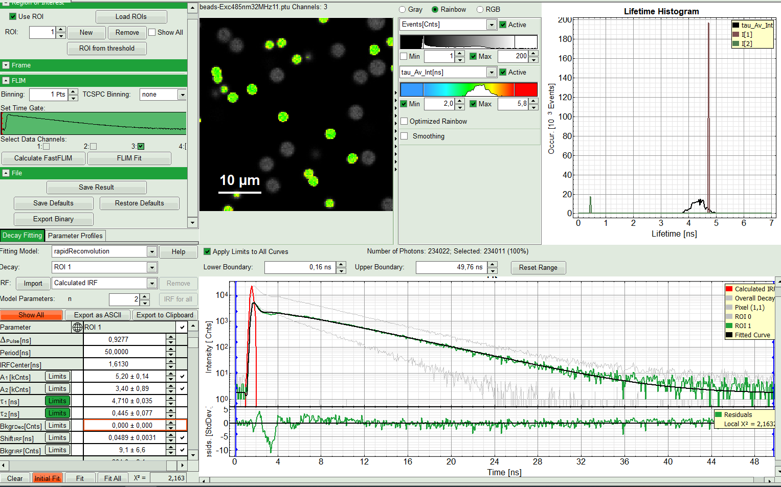
The fitting quality gets better, although there is still a bit of deviation in the residuals after the IRF in the decay window. This however can be explained as a systematic error. Nevertheless we can test it with three components.
Response:
At the first glance the fit does not look significantly better. With closer look in fitting table, you see a third comportment appears with a negative amplitude which physically is impossible. That means a fit with two components gives the best result. As it was the same for both ROIs, we can now apply this model on both ROIs by “Fit All”.
If you wanted to measure the lifetime of the beads, you have reached your goal, can save the results and finish the analysis at this step.
Perform a pixel-by-pixel Fit and save results
- If you are also interested in other information e.g. the spread of the mean lifetime from pixel to pixel for similar beads, you can proceed the following way:
- Get back to “Decay Fitting” window. Select ROI 0, fix the lifetimes by unchecking them in the fit table, as well as the IRF background and IRF Fit.
- One the single pixel level, the background can be neglected, and the parameter “Backgroudn Decay” can be fixed to 0 in this example.
- Set constraints for A1 and A2, so they cannot become negative.
- and press “FLIM fit”.
Response:
The image and the histogram will get updated. The rainbow scale contains now the fitted, intensity weighted mean lifetime, instead of the “fast Lifetime”, based on the photon arrival time only. The Histogram on the right of the image contains now the photon weighted distribution of the intensity-weighted mean lifetime. The distributions for lifetime component 1 and lifetime component 2 appear as bars, as these parameters have been fixed in the pixel-by-pixel fit. Now you can save the analysis by clicking “save results”.
Response:
The result file with default name of “FLIM.pqres” will appear on the list on the left hand.
- Repeat these steps for ROI 1. Fix lifetimes and press “FLIM Fit”.
- If you compare the result image after the fit with the fast lifetime image above, you will see that the lifetime distribution of the lifetime within a single bead is much more uniform, as effects due to background as well as decay distortions causes by the high countrate have been corrected for.
- If you want to export the lifetime distribution, open the context menu via right mouse click, when the mouse pointer is over the lifetime distribution graph.
- Press “Save Result”. The old result file is not overwritten, but a new result-file is created.
- Use a two slow clicks on FLIM result files (.pqres) to rename them properly.
