How to Work with Instrument Response Functions (IRFs) Measured with a Microscope

IRF stands for Instrument Response Function, and it reflects how a component with an infinitive short lifetime is seen by the instrument. Of course, all components of the instrument contribute to both shape and width of the IRF. This width is an indicator the timing resolution of the instrument.

The IRF width is approx. a quadratic sum of the widths of all contributions. The observed decay in a time domain measurement is a convolution of the 'real' decay with the IRF. Therefore for accurate measurements of lifetimes, especially near to the timing resolution, the instrument response function (IRF) should be taken into account. For IRF Measurements, several strategies are possible which are described here: https://www.tcspc.com/doku.php/howto:how_to_measure_the_instrument_response_function_irf

For the further analysis it is assumed that:

• the settings have been done in the same way as for a FLIM measurement. This way the IRF can be monitored by the PicoQuant detectors.
• the count rate should be kept lower than for a normal FLIM measurement (see Differential Count Rate).

• It is important that the “Laser Power” output is not changed at the PDL or SEPIA laser driver or in the setting of the (LSM) software. Changing the electrical power of the laser changes the shape and temporal position of the laser pulse. ¹⁾
• The measurement has been stopped, when the decay histogram in the TCSPC preview has reached ~10000 counts in the peak channel.

For IRF Measurements, several strategies are possible which are described here.

1. First the measured IRF needs to be made accessible for being used in the analysis. Therefore, highlight the file with the measured IRF (single mouse click on the .ptu-file)
An example measured IRF can be found in Tutorials workspace https://figshare.com/s/4957fcfa684daef86c23.
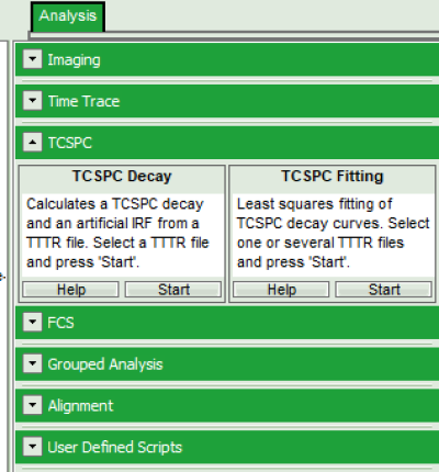
2. In Analysis tab, under TCSPC, find `TCSPC Decay`. Click Start;

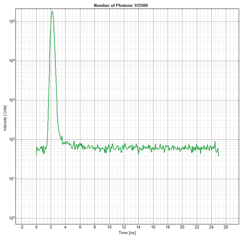
Response: you see this kind of curve: (Before selecting a detection channel the peak is above 100000, so fine for this step)
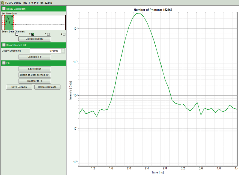
3. Select the proper detection channel (1 or 2) and Click”Calculate Decay”. The decay is then updated.
4. Select the decay range by Setting a `Time Gate` (move the red bars) to limit the decay the area where this has an impact.

Note:

• The green area is used for the timegate.

• In order to define the time range better, double click on the graph with the gating selection. It is opened in a new window with you can enlarge in order to define the time gates better. When content, click o.k.

• Decays with quenched components for IRF-measurments as described here can also be used for IRF-fitting without time gating. However, as these decays contain the noise of the complete TCSPC-window, the end of the fitting curve might show noise fluctuations.

Setting a time gate removes the noise, and the fit curves usually become smoother.

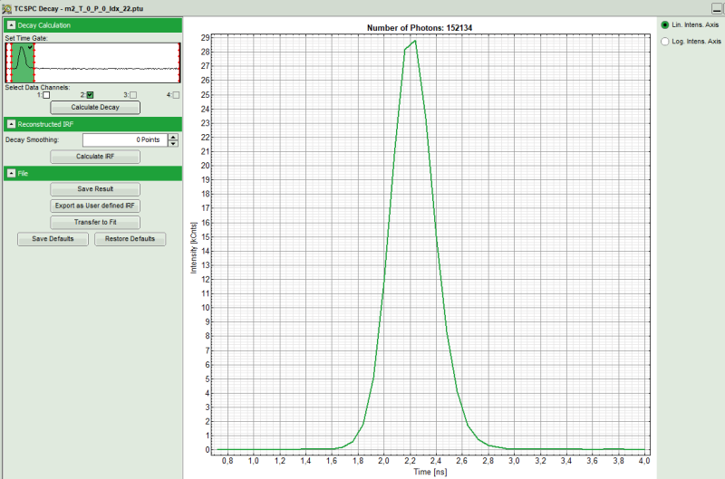
5. Then click again on `Calculate Decay`. As a result you will see:

6. Click on “Export Decay as IRF”. Rename the file accordingly. The IRF can now be used for the fitting.

Note:

• In general, an indicator of the achievable time resolution of the system is the FWHM (full width of half maximum) of an IRF-measurement. For PicoQuant systems it´s usually in the range of 100-400 ps, depending on detector, electronics and laser settings (Please see `System Specification File` which is left by installation in your lab. The main influence is due to the settings of the PDL or SEPIA-Unit, as operating the laser with full power will increase the pulse width and IRF. Also the type of detector is important. Finally the type of TCSPC-unit used has an influence. Apart from the laser (unless you use a TiSa), however, all the other factors can be considered constant. For SPAD detectors, the IRF also depends on the detection wavelength).

Select the linear range for measured curve (on top right), right click, activate `Data Reader`, and try to find FWHM and see how broad it is. ²⁾

In this example channel 2 was selected, now the data can be “saved as IRF”, and be imported for future analysis accordingly. Please check the different FLIM-related tutorials for more information about the fitting.